Happy holidays, everyone! The following is part question, part visual gallery, and part classical mechanics problem. Inspired by snow over the weekend I began simulating the vibrations of the following hexagonal lattice system:
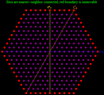
The 271 purple dots represent point masses of mass $m=1$ and are spaced apart by a spacing $a=1$, and each point mass is connected to each of its six nearest neighbors via springs with rest length $L=1$ and spring constant $k$. The red dots are fixed in place, and essentially act as an immovable boundary condition, while the purple dots are free to move horizontally and vertically in the plane. The lattice has $D_{6}$ symmetry, and three of the elements (vertical reflection $\sigma_v$, horizontal reflection $\sigma_h$, and $\pi/3$ rotation $C_6$) are shown for reference.
The entire system potential becomes $$U(\mathbf{r})=\sum_{i,j}\frac{1}{2}k\left(L-\left|(\mathbf{r}_i^{e}+\mathbf{r}_i)-(\mathbf{r}_j^{e}+\mathbf{r}_j)\right|\right)^2$$ where $$\mathbf{r}=(\mathbf{r}_1,\mathbf{r}_2,...,\mathbf{r}_{271})^\mathsf{T}=(x_1,y_1,x_2,y_2,...,x_{271},y_{271})^\mathsf{T}$$ is the vector which represents the state of deformation of the system away from the equilibrium configuration $\mathbf{r}^e$ in the image above ($\mathbf{r}_i$ represents the vector displacement of the $i$th point from equilibrium), and where the sum runs over nearest-neighbor pairs.
As per the usual normal mode analysis, it's easy to show that $U(\mathbf{0})=0$ and $\nabla U(\mathbf{0})=\mathbf{0}$, and thus the system admits the second-order Taylor expansion
$$U(\mathbf{r})=\mathbf{r}^\mathsf{T}\mbox{H}\mathbf{r}+O\left(\mathbf{r}^3\right)$$ where $$\mbox{H}=\nabla\nabla U(\mathbf{0})$$ is the $542 \times 542$ Hessian matrix of the potential at equilibrium. For small oscillations, the normal mode picture is applicable, and the eigenvibrations are the columns of the orthonormal eigenbasis $\Lambda$ of $\mbox{H}$. $\mbox{H}$ has a closed-form block matrix expression, although I omit it here for brevity.
Note that $$U(\mathbf{r})=U(\Gamma_g\mathbf{r})$$ for all $\mathbf{r}$ and for all $g\in D_6$ where $\Gamma_g$ is the matrix representation of the symmetry operation $g$- for example, $\Gamma_{C_6}$ is the block matrix that maps every coordinate to the one 60 degrees CCW rotated from it, and also rotates each vector by 60 degrees. Since $U(\mathbf{r})=U(\Gamma_g\mathbf{r})$, we can take derivatives twice to obtain $$\nabla\nabla U(\mathbf{r})=\Gamma_g^\mathsf{T}\nabla\nabla U(\Gamma_g\mathbf{r})\Gamma_g.$$ By noting that $\Gamma_g^\mathsf{T}=\Gamma_g^{-1}$ for all $g\in D_6$ and setting $\mathbf{r}=0$, we obtain $$\Gamma_g\mbox{H}=\mbox{H}\Gamma_g$$ and hence $$[\mbox{H},\Gamma_{D_6}]=0.$$
Mathematica revealed that 180 of the 542 eigenstates $\Lambda_k$ of $H$ were singly-degenerate. As is well-known, a singly-degenerate eigenstate of a matrix $\mbox{H}$ is automatically an eigenstate of any $\mbox{A}$ for which $[\mbox{H},\mbox{A}]=0$, and thus all 180 singly-degenerate vibrations satisfy $$\Gamma_g\Lambda_k=\lambda_k^g\Lambda_k$$ and thus manifest in numerical outputs as strikingly beautiful patterns, which I'll show in a second. In particular, they are eigenstates of $\sigma_v,\sigma_h,C_6$ and the inversion operator $i$.
Meanwhile, the other 362 eigenstates are doubly degenerate and so Mathematica simply spits out an arbitrary pair spanning each eigenspace, so they don't look very nice. However, they can be "symmetry-projected" via the usual means, which I experimentally found was best done by choosing the pair to be a simultaneous eigenbasis of $\mbox{H}$ and $\Gamma_{\sigma_v}$ (which, again, can be done since $[\mbox{H},\Gamma_G]=0$). Likewise, since $\sigma_v$ commutes with $\sigma_h$, they are also in a definite eigenstate of $\sigma_h$, and by extension, eigenstates of $i=\sigma_v\sigma_h$. However, they are not necessarily eigenstates of rotation $C_6$ since $C_6$ doesn't commute with reflections. As a cheap aesthetic surrogate, I define "generalized" eigenvalues as $$\lambda_k^{g}=\left<\Lambda_k,\Gamma_{g}\Lambda_k\right>,$$ which gives the correct result whenever $\Lambda_k$ is an eigenstate of $g$, and gives a sort of average value when it is not.
The 542 symmetry-classified vibrations were visualized in Mathematica and exported as a gigantic 5343 x 8913 pixel image. Here is a considerably smaller preview image (it's far too small to read the words, click the full-size to see everything in detail):
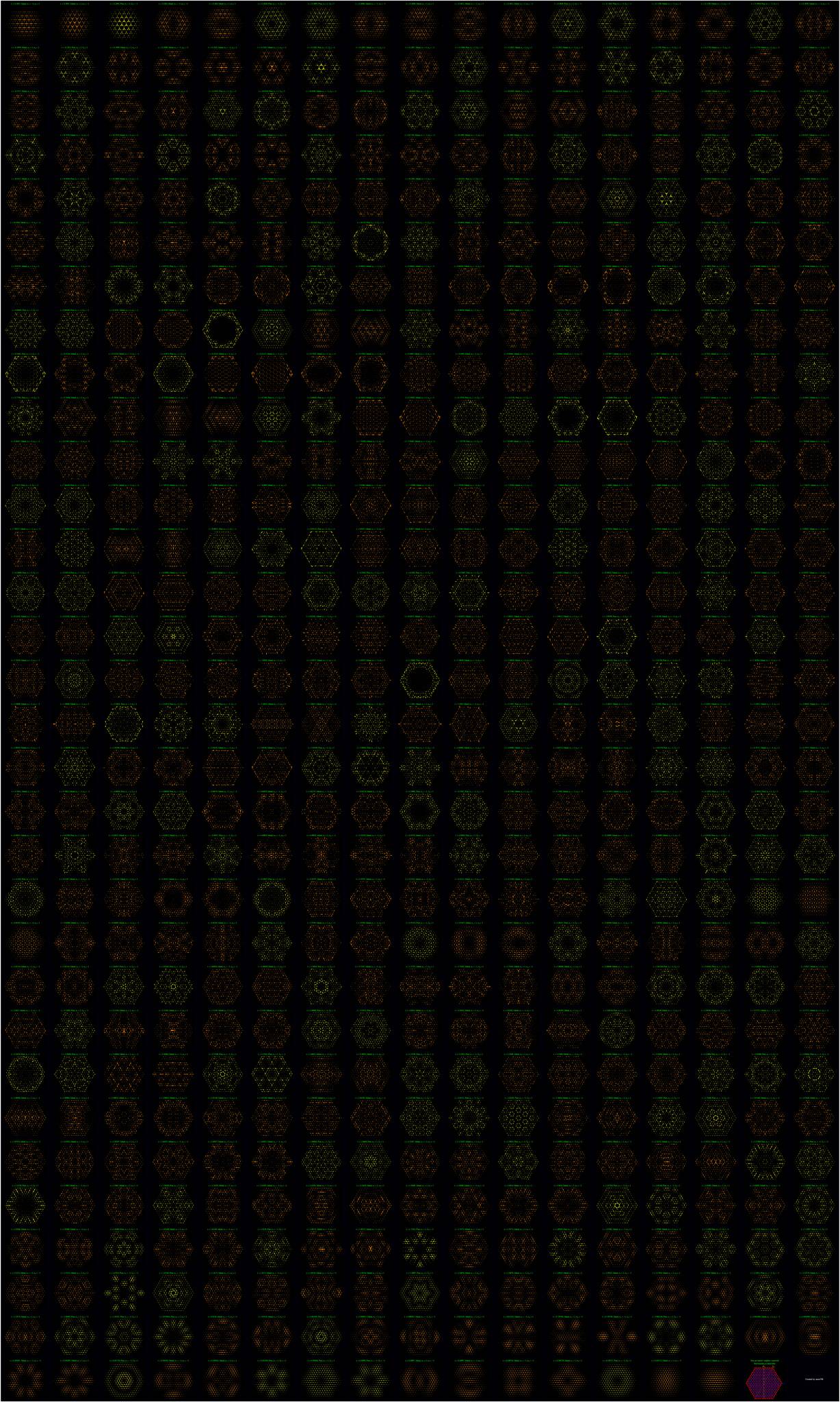
They've been color-coded, with the yellow ones being singly-degenerate ("pure") and the orange ones being doubly-degenerate ("mixed"), their eigenvalue of $\mbox{H}$ is given ("$\lambda$"), and their symmetry numbers with respect to the four symmetry operations I've mentioned is also given. They're ordered by vibrational frequency, from highest to lowest. Many of them are reminiscent of snowflakes when viewed at lower resolution, which I thought was kind of pretty.
At this point, all I've done is just compute a bunch of normal modes, which are valid for small oscillations. For large-amplitude vibrations, anharmonic coupling effects come into play, mixing the modes together and distorting their frequencies. To visualize this nonlinear mixing process, I numerically simulated the system starting out displaced in the direction of a single eigenmode, but with large vibrational amplitude. The time-varying vector output $\mathbf{r}(t)$ from NDSolve was then converted into the symmetry-adapted eigenbasis as $$\mathbf{r}'(t)=\Lambda^\mathsf{T}\mathbf{r}(t)$$ to yield the "population" in each eigenmode over time, and the result was plotted using ArrayPlot. For visual simplicity, I used a smaller 37-point lattice, rather than the 271-point lattice I've been using previously, although the same code can be used interchangeably for both.
For example, starting in one of the $(C_6,\sigma_v,\sigma_h,i)=(-1,-1,1,-1)$ symmetry states with an amplitude such that the points traveled a distance of about 1/8 (ie, smaller than lattice displacement, but still reasonably large) yielded the following:
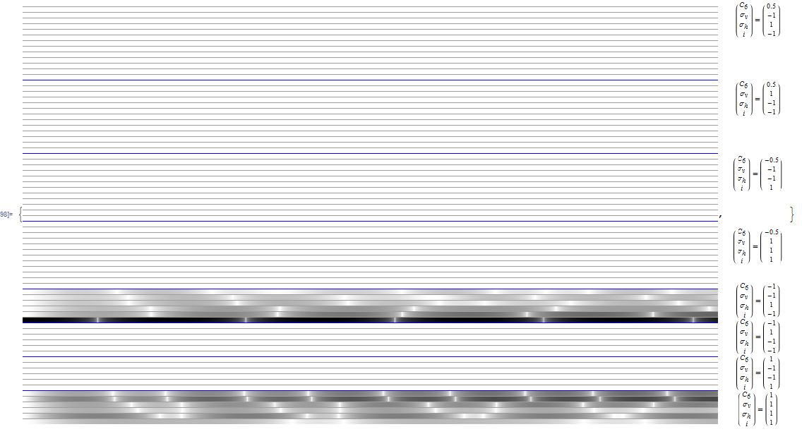
The $x$-axis is time (from left to right), and each of the 74 horizontal bars represents an eigenmode, which have been grouped together by which of the 8 symmetries it belongs to. White indicates no amplitude, black indicates large amplitude, and the color scale is somewhat logarithmic to make things easier to see. As can be seen, near the very beginning amplitude gets mixed into other states, but the mixing is confined to states with $(-1,-1,1,-1)$ symmetry or $(1,1,1,1)$ symmetry only. Similarly, repeating this with a $(\frac{1}{2},-1,1,-1)$ symmetry state yielded the following:
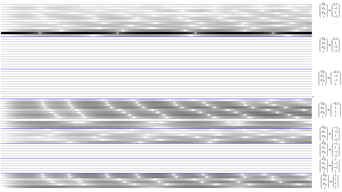
This time, the coupling is limited to four symmetry classes. I found that coupling only depended on symmetry, which I'm sure people more knowledgeable than myself will know well. Finally, I noted that such symmetry restrictions would spontaneously lift themselves at extremely large displacements without warning after some time; the time at which the sudden change occurred was strongly dependent on the precision of the numerical solver, and random noise added to the initial conditions caused an immediate breaking of symmetry. Here is an example of such a phenomenon:
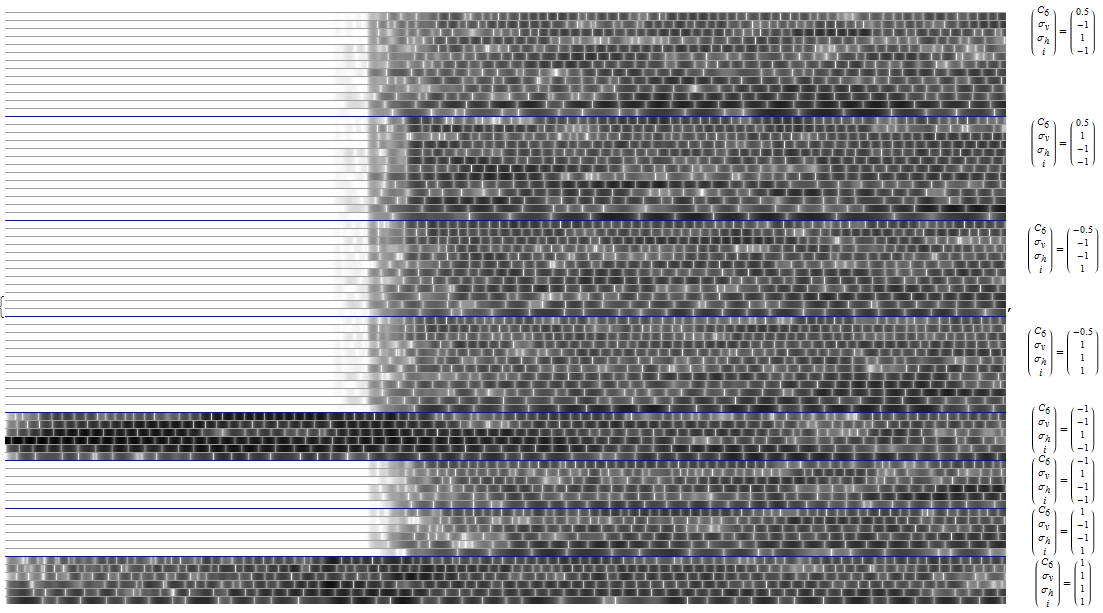
Here's a question: is this an classical-mechanical example of spontaneous symmetry breaking? It seems that the system starts out in a state of definite symmetry, but that upon provocation by numerical noise, population 'tips over the edge' and spills into the rest of the symmetry classes, equalizing everything.
Here's another question. I found that coupling was nonreciprocal, in the sense that population from $(1,-1,-1,1)$ modes could spill into modes of $(1,1,1,1)$ symmetry, but that the reverse was not possible (ie, the flow of amplitude seems to have sources and sinks). To be more specific, the coupling directions looked like this:
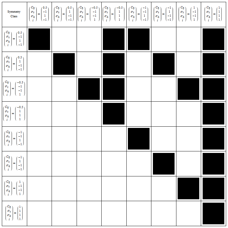
If the $i,j$ entry is black, then energy can couple from symmetry class $i$ to symmetry class $j$, and if it's white, it's forbidden (with the exception of when spontaneous breaks occur at extreme amplitudes). Note that not only is it upper triangular with the way I ordered the symmetry blocks here, but it's actually a $2\times 2$ block matrix of the form $$\left(\begin{array}{cc} A & A\\ 0 & A \end{array}\right)$$ where $A$ is a $4\times 4$ matrix which is also upper-triangular. Does anybody have any idea how or why this happens? I have to admit it's all a bit over my head. I did all of this intending to print out posters as a Christmas present for my parents, but I noticed all this wacky stuff in the process. I suspect it's some kind of weird "classical mechanics selection rule" but I'm not very good at algebra, so the reasons are all opaque to me, and I haven't formally taken classical mechanics.
As a final example of pretty pictures, I should point out that my choice of symmetry projection for the doubly-degenerate modes was in a realistic one, as it matches the eigenmodes of the corresponding lattice with a unitary horizontal shear transformation applied to the equilibrium positions in the limit as the shear matrix approaches the identity matrix. To be specific, applying the shear transform $$\left(\begin{array}{cc} \frac{x}{1-x} & 0\\ 0 & \frac{1-x}{x} \end{array}\right)$$ to the lattice and computing the eigenfrequencies as a function of $x$ yielded the following beautiful pattern:
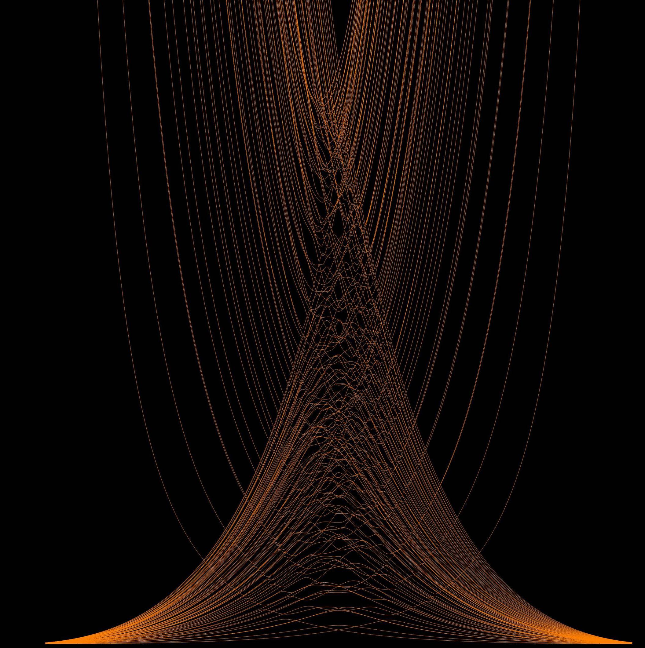
It's available in higher resolution here. The $x$-axis is $x$, and each line represents an eigenfrequency. They have lots of crossings and avoided crossings, reminiscent of Stark effect perturbations in atoms. In the limit as $x\rightarrow\frac{1}{2}$, the eigenstates of $\mbox{H}$ approach the symmetry-adapted ones.
