Physical meaning of Legendre transformation

Question

I would like to know the physical meaning of the Legendre transformation, if there is any? I've used it in thermodynamics and classical mechanics and it seemed only a change of coordinates?

Answer 1

Legendre transformations are commonly used in thermodynamics (to switch between different independent variables) and classical mechanics (to switch between the Lagrange and Hamilton formalisms). But you rightly ask: what exactly is a Legendre transformation? Where does it come from? What makes it work?

In (1D) classical mechanics, for example: if we have a Lagrangian $L(q,\dot{q}[,t])$, why can we define a variable

$$p = \frac{\partial L}{\partial\dot{q}}$$

and expect to be able to construct a new function (the Hamiltonian) $$H(q,p[,t]) = p\dot{q}-L(q,\dot{q}[,t])$$ that behaves well? What's the relationship between both functions?

Let's look at the Lagrangian and Hamiltonian as a guiding example. I'll keep it fairly abstract/general, but the notation of Lagrangian/Hamiltonian can help make things more concrete and clearer.

One thing I will do, however, is leave out the explicit time dependence. It's not important to our analysis and more often than not there will indeed be no explicit time dependence. Furthermore, I'll denote $v\equiv\dot{q}$ to put less emphasis on the relation to $q$, since it is not important for the Legendre transformation.

So what do we need for a Legendre transformation?

Well, first of all we need two variables $v$, $p$ that are single-valued functions of each other. Another way to put this is that $p$ must be a monotone function of $v$ and vice versa. Figure 1 shows an example of such a function.

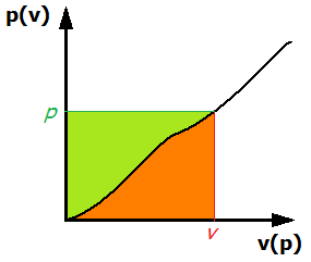
Figure 1. Example of a single-valued relation between $v$ and $p$.

For such variables it is always possible to construct a pair of functions with the property that differentiation of one of the functions with respect to one of the variables yields the second variable. Equivalently, the derivative of the second function with respect to this second variable yields the first variable.

In our example of classical mechanics, the functions we can construct for our two variables $v$ and $p$ are the Lagrangian $L(q,v)$ and the Hamiltonian $H(q,p)$.$^1$ They satisfy (by definition) the differential relations

$$\begin{align} \frac{\partial L}{\partial v} &= p \\ \frac{\partial H}{\partial p} &= v \end{align}$$

Why does it work?

Indeed, why can we construct such functions? Take another look at figure 1. The way the graph is set up, it looks like a graph of $p$ as a function of $v$. So if we integrate this function between $0$ and some value $v$ (shown on the graph), the answer we get is the orange area under the curve. This integral is our first function! Indeed, if we return to the notation of our classical example (I'm going to leave out the $q$ dependence from now on):

$$L(v) = \int_0^v{p(v')dv'}$$

because

$$\frac{\partial L}{\partial v} = \frac{\partial}{\partial v}\int_0^v{p(v')dv'} = p.$$

Now if we consider the curve in Figure 1 to be $v$ as a function of $p$ (rotate the graph around if that makes it clearer to you), we can make a similar reasoning. This time we integrate between $0$ and $p$ where $p$ has been chosen to correspond to our earlier $v$.$^2$ This integral is our second function; so in terms of our 1D classical example:

$$H(p) = \int_0^p{v(p')dp'}.$$

You may have noticed that we've described a rectangle with the integrals (and therefore the two functions $L$ and $H$). This rectangle has a total surface of $p\cdot v$. But we've also calculated its surface in two parts: the green and the orange. The sum of both must therefore be equal to $pv$. This yields the Legendre transformation

$$L(v) + H(p) = pv$$

or

$$H(p) = pv - L(v)$$.

How does a Legendre transformation work in practice?

Here's a 3 step plan:

1. Start with your first function, e.g. $L(v)$. $\left[\right.$or $U(S)$ for a thermodynamical example$\left.\right]$

2. Find the conjugate variable by differentiation:

   $$p = \frac{\partial L}{\partial v} \hspace{2cm} \left[T = \frac{\partial U}{\partial S}\right]$$

3. Construct the second function

   $$H(p) = p\cdot v - L(v) \hspace{2cm} \left[\left(-F(T)\right) = T\cdot S - U(S)\right]$$

   and insert the conjugate variable wherever you can, i.e. replace $v$ $[S]$ with the expression $v(p)$ $[S(T)]$ throughout the entire expression.

Partly from Figure 1, it should now be clear that the two functions are not only generally different from each other, they describe things from a different perspective (we had to view the curve in Figure 1 once as a function $p(v)$ and once as a function $v(p)$). The functions are complementary and their close relation is governed by a Legendre transformation.

---

$^1$ These are also functions of $q$, but that's not important. They could be functions of any number of distinct variables, though their list of variables will obviously be the same except for $v$ and $p$. Indeed, the Legendre transform doesn't change any of the other dependencies. If this is not clear now, it should become so throughout the rest of this explanation.

$^2$ Note that this is where the single-valuedness of the relation between $v$ and $p$ is required. If $v(p)$ was a parabola for example, then there would be ambiguity about which $p$ corresponds to the $v$ we used.

Answer 2

I find the convex-analysis interpretation of the Legendre transform to be the most enlightening.

(this is an adaptation of a blog post I wrote for a website that has since been deleted)

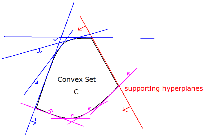
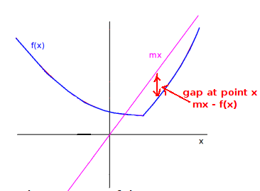
A convex set is uniquely determined by it's supporting hyperplanes. The Legendre transform is an encoding of the convex hull of a function's epigraph in terms of it's supporting hyperplanes. If the function is convex and differentiable, then the supporting hyperplanes correspond to the derivative at each point, so the Legendre transform is a reencoding of a function's information in terms of it's derivative.

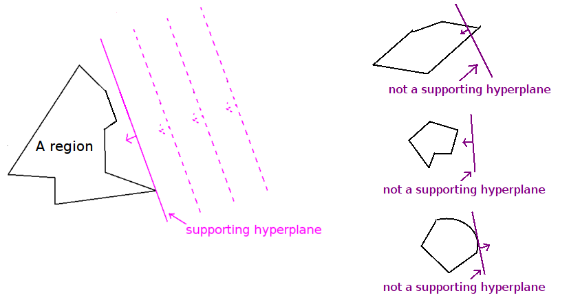
A supporting hyperplane of a region is the closest possible oriented hyperplane to that region, among all hyperplanes with a given normal, such that all points in that region reside on the outside of the hyperplane.

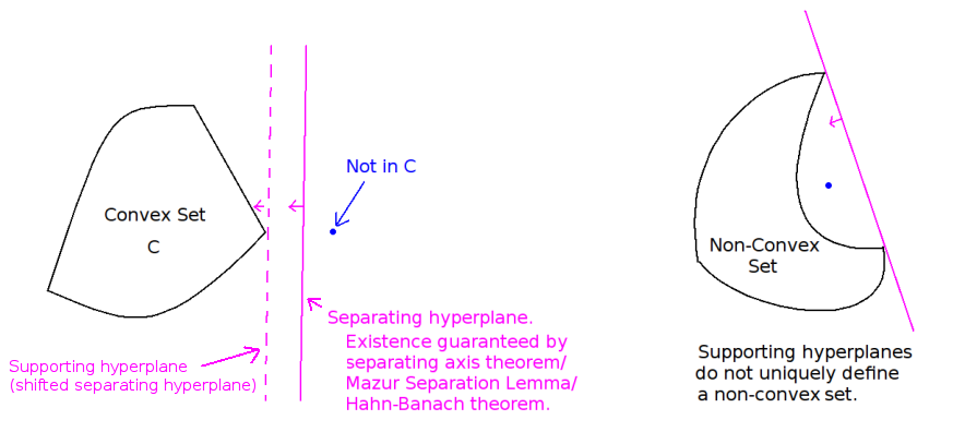
A closed convex set is uniquely determined by its supporting hyperplanes.

Why? No supporting hyperplane can "cut into" the set that it supports, and for each point outside the set, there exists a hyperplane that separates it from the set.

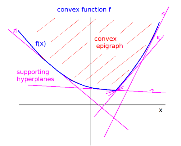
A closed convex function is uniquely determined by its lower supporting hyperplanes.

The Legendre transform, $f^*$, is an encoding of a function $f$'s supporting hyperplanes.

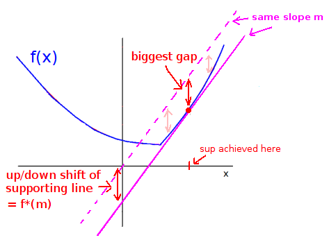
In 1 dimension ($f:\mathbb{R}\rightarrow \mathbb{R}$), the Legendre transform is $$f^*(m) := \sup_{x \in \mathbb{R}} ~ (mx - f(x)).$$

• The argument of the supremum is the gap between the function, and a line with slope $m$.

• The supremum is achieved where the supporting line barely touches $f$'s graph.

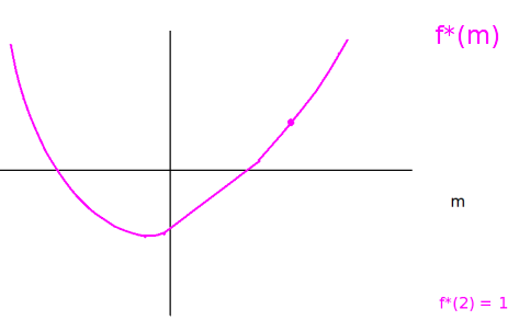
• $f^*$ encodes all of the information about $f$'s supporting lines. You give $f^*$ a slope, $m$, and $f^*(m)$ tells you how far to shift a line with slope $m$ up or down, so that it just barely touches the graph of $f$.

In n dimensions ($f:\mathbb{R}^n\rightarrow \mathbb{R}$),

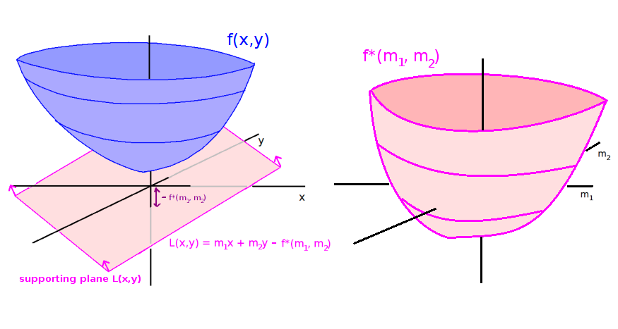
$$f^*(\mathbf{m}) := \sup_{\mathbf{x} \in \mathbb{R}^n} ~ (\langle \mathbf{m}, \mathbf{x}\rangle - f(\mathbf{x})),$$ where $\langle \cdot, \cdot \rangle$ is the inner product.

If $\mathbf{m} = (m_1, m_2, \dots, m_n)$ is a vector of slopes, then $f^*(\mathbf{m})$ is the up/down shift of the hyperplane with directional slopes $(m_1, m_2, \dots, m_n)$, such that the hyperplane just barely touches the graph of $f$.

$f^*$ encodes the information about all of $f$'s supporting hyperplanes. you give $f^*$ a slope vector $\mathbf{m}$, and $f^*(\mathbf{m})$ tells you how far to shift the hyperplane with slope vector $\mathbf{m}$ up or down so that it just barely touches the graph of $f$.

Here are some other links that discuss this convex analysis perspective of the Legendre transform:

http://jmanton.wordpress.com/2010/11/21/introduction-to-the-legendre-transform/ (great in-depth explanation)

http://www.mia.uni-saarland.de/Teaching/NAIA07/naia07_h3_slides.pdf

---

As an aside, this intuition also extendes to infinite dimensions. That is, $f:X \rightarrow \mathbb{R}$, where $X$ is a Banach space. There the Legendre transform is $$f^*(\phi) := (\phi(x) - f(x)),$$ where $\phi$ is a linear functional. The idea of a hyperplane is less clear, but one might think of $\text{ker}(\phi) + b$ as a generalization of a hyperplane offset by height $b$ from the origin.

Answer 3

See

http://en.wikipedia.org/wiki/Legendre_transformation#Applications

In theoretical physics, the basic or defining mathematical properties of the Legendre transformation are used to switch between one form of the energy - or "potential", as the generalized energies are called in thermodynamics - to another.

This is important to switch between the Lagrangian in abstract mechanics that depends on $x,v$ (positions and velocities) to the Hamiltonian, the true energy that depends on $x,p$.

In thermodynamics, the number of applications and "types of switches" is even higher. You may go from energy to enthalpy or Helmholtz free energy or Gibbs free energy by Legendre-transforming with respect to various variables. The transform goes back and forth. As the Wikipedia example explains, there are other useful variables that you may Legendre-transform with respect to, including the charge and voltage.

You may consider the Legendre transformation to be a "mere" redefinition of variables - but that's why it's so important in practice. In reality, the different ways to describe the system that differ by a Legendre transformation are "equally fundamental" or "equally natural" so it's often useful to be familiar with all of them and to know what is the relationship between them. The relationship is given by the Legendre transformation.

Answer 4

There are already some nice answers regarding intuitive interpretations of the Legendre transform. What I want to contribute here, is a more physical reason/motivation for why they appear. I.e., instead of focusing on their physical interpretation, I will focus on the physical requirements that uniquely define Legendre transforms. This explains why you would inevitably end up inventing them, even if you had never heard of them before.

Variational principles are fundamental to physics. Legendre transforms naturally arise when requiring that variational principles carry over when changing variables; in fact, they turn out to be the unique solution to this physical requirement. I will illustrate this in the thermodynamic context. (A main conceptual difference from the other explanations on this page, is that according to this view, it is important that our function also depends on other variables in order to naturally arive at Legendre transforms!)

One important instance of a variational principle is the principle of minimum energy: a closed system with a fixed entropy will minimize its energy (note that 'closed' means that there is no mass transfer, but energy transfer is allowed!). This can be derived from the second law of thermodynamics; for a derivation, see here. To state this more precisely: if we denote our internal energy $U(S,X)$ where $S$ is the entropy and $X$ is some macrosopic variable that can thermalize (i.e., it is not fixed; e.g., a density profile, or the position of a sliding partition), then in equilibrium, we have $$ \boxed{ \left. \frac{\mathrm dU(S,X)}{\mathrm dX} \right|_{S} = 0 } \quad \textrm{(for the equilibrium value $X= X_\textrm{eq}$).} $$ (I will be suppressing other thermodynamic variables that might be held fixed, such as volume.) Here I am following the notational convention that the bar indicates what one is holding fixed when taking the derivative.

To each extensive thermodynamic variable, such as entropy, we can associate an intensive variable, in this case the temperature: $$ T(S,X) \equiv \left. \frac{\mathrm dU(S,X)}{\mathrm dS} \right|_{X}. $$ Such associated extensive and intensive variables are said to be conjugate.

Depending on the physical context, it can be more natural to keep the intensive parameter $T$ fixed, rather than the entropy $S$ (e.g., for a system connected to a heat bath). In principle (if $U(S,X)$ is convex as a function of $S$), we can invert the above relationship to obtain $S(T,X)$. We can thus express the internal energy as a function of $T$ and $X$, i.e., $U(T,X) \equiv U(S(T,X),X)$. However, we have lost our variational principle: equilibrium no longer corresponds to a zero derivative! Indeed, by the chain rule, $$ \left. \frac{\mathrm dU(T,X)}{\mathrm dX} \right|_{T} = \underbrace{ \left. \frac{\mathrm dU(S,X)}{\mathrm dS} \right|_{X}}_{= \; T} \left. \frac{\mathrm dS(T,X)}{\mathrm dX} \right|_{T} + \boxed{ \left. \frac{\mathrm dU(S,X)}{\mathrm dX} \right|_{S} }. $$ Note that the boxed term is the one that is zero at equilibrium. Hence, when expressing the internal energy as a function of $T$ instead of $S$, our equilibrium condition has become $$ \boxed{ \left. \frac{\mathrm dU(T,X)}{\mathrm dX} \right|_{T} = T \left. \frac{\mathrm dS(T,X)}{\mathrm dX} \right|_{T} } \quad \textrm{(for the equilibrium value $X= X_\textrm{eq}$).} $$ This is clearly annoying: it would be much nicer to have a single function which is extremized at equilibrium, rather than having to match the gradients of different functions! However, since the derivatives are with respect to fixed $T$, we can move it inside the derivative. Hence, moving everything to one side, we have $$ \boxed{ \left. \frac{\mathrm d \left( U(T,X) - T \;S(T,X) \right)}{\mathrm dX} \right|_{T} = 0 } \quad \textrm{(for the equilibrium value $X= X_\textrm{eq}$).} $$

Defining $F(T,X) \equiv U(T,X) - T \; S(T,X)$ (which you might recognize as the (negative) Legendre transform!), we thus see that this is the appropriate quantity to variationally extremize when keeping temperature fixed! More generally, the above actually shows that $$ \boxed{ \left. \frac{\mathrm dF(T,X)}{\mathrm dX} \right|_{T} = \left. \frac{\mathrm dU(S,X)}{\mathrm dX} \right|_{S} }, $$ for any value of $X$. If we enforce this as our physical requirement, then the above can be read as a proof that this uniquely gives the above $F(T,X)$ (called the Helmholtz free energy) up to an arbitrary function $f(T)$ (which is independent of $X$). To kill this remaining arbitrariness, we can in addition note that if we go for the aforementioned minimal choice of $F(T,X)$, then we have the pleasant property that (exercise) $$ S(T,X) \equiv -\left. \frac{\mathrm dF(T,X)}{\mathrm dT} \right|_{X}. $$ In other words: just as the derivative of the internal energy w.r.t. entropy gives us temperature, the derivative of the free energy w.r.t. temperature gives us the entropy (note that requiring this property forces our above unknown function to be constant: $f(T) = \textrm{cst}$). The significance of this is that it makes the whole process an involution! I.e., if we use $F(T,X)$ as our original starting point and feed it in at the top, we will end up with $U(S,X)$ as the result (possibly up to an irrelevant constant). In particular, this means that $F(T,X)$ and $U(S,X)$ carry the same information!

In summary, when the derivative w.r.t. the original variable is taking as the new variable, the Legendre transform naturally arises as the (virtually) unique function satisfying the constraints that (1) the derivatives w.r.t. other variables agree and that (2) the derivative of the new function w.r.t. the new variable gives back the original variable!