1
$\begingroup$

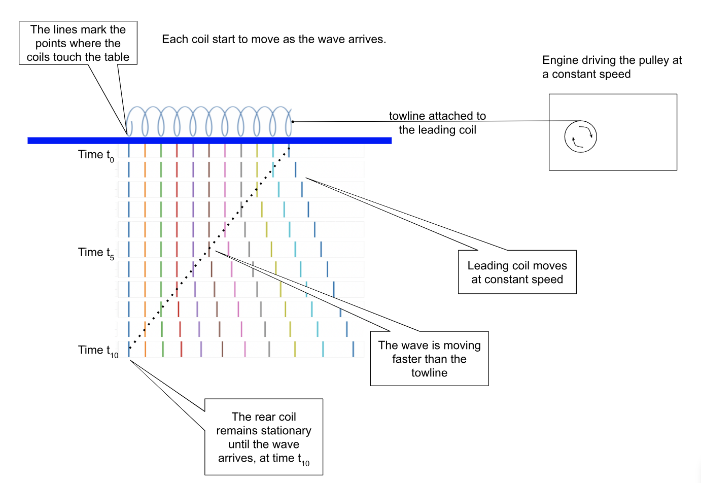
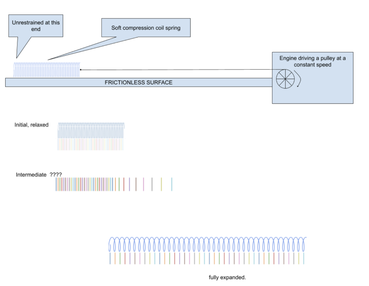
Could you explain the coil behaviour from the moment the pull begins until the entire coil starts to move? Diagram of setup

There are explanations and videos about falling slinkys, but those are complicated by gravity working longitudinally instead of transversely as in my example and they are not compression coils.
Eventually, the rear of the coil will start to move, but there is an intermediate period of time in which the front of the coil is moving before the back starts to move.
I suspect that the time before the back of the coil starts to move is determined by the speed of transmission of a "rarefaction wave" in the coil, and I would like to know how long the intermediate phase is.
[EDIT 1] a) The material of the spring is not massless. It has a non-zero linear density.
b) I am aware that once the back of the spring starts to move, the dynamics change and the spring will probably start to oscillate, but I'm only interested in the behaviour up to that point in time.
[EDIT 2] I'm after an explanation of how the spring behaves, ultimately so I can code it (python), so, in programming terms, I guess I'm asking for the algorithm that would replicate/ emulate/simulate the behaviour. Specifically, I'd like to understand how to calculate the time interval for this intermediate phase, considering factors like: speed of the front coil, number of coils, the pitch of the coil, the linear density of the spring wire, the spring constant of the coil etc. etc.
It might be simpler to assume a value for the speed of the front coil as a fraction of the speed of the (low) pressure wave through the spring. That way would eliminate the complications of linear density, elasticity etc.
I know it's a big ask, so I'm hoping to leverage any existing work.

$\endgroup$
4
  • $\begingroup$ Is this supposed to be a massless spring? $\endgroup$
    – Bob D
    Commented May 9 at 22:48
  • $\begingroup$ @BobD Fair question, not massless, please see edit. $\endgroup$ Commented May 9 at 22:54
  • $\begingroup$ Are you looking for a quantitative answer or qualitative answer? I can write a program later tongiht to get a visual if that would answer your question. $\endgroup$
    – Nic
    Commented May 10 at 4:04
  • $\begingroup$ @Nic Yes I wasn't very clear about my expectations. Please see [EDIT 2] where I have attempted to clarify that. $\endgroup$ Commented May 10 at 7:25

2 Answers 2

0
$\begingroup$

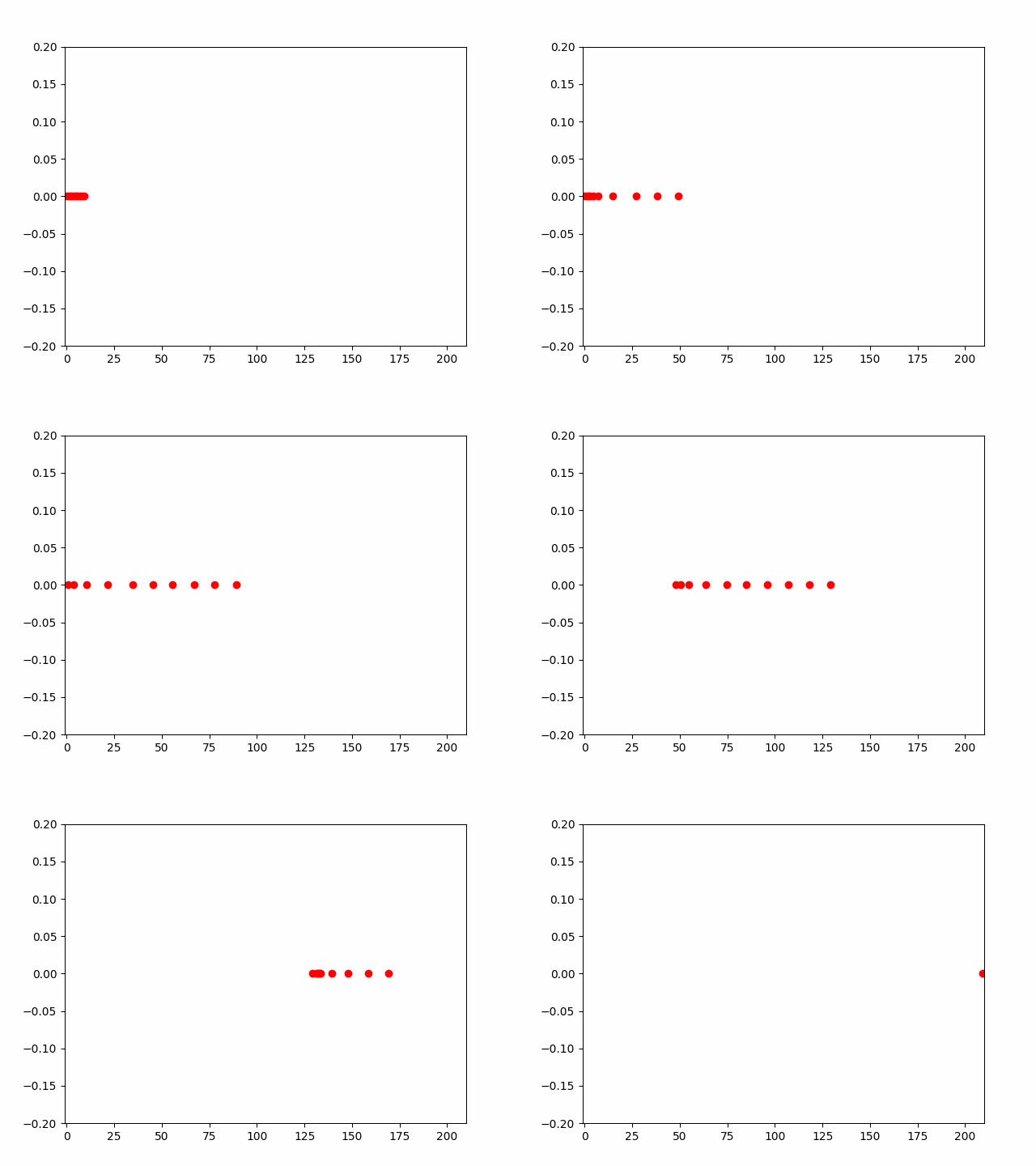
Sorry it took me a while to get to this. But effectively, we can model it as a bunch of mass and springs where the first mass is forced to move at a constant speed. Then, we can take the limit as the number of springs gets larger and closer together as the answer to your question. I coded a simulation for this in python and I will share the result and my code below. Feel free to comment on questions or advice on how to make my simulation better as I am always looking for ways to improve.

Some analytical comments: we can see that about halfway through the gif all the dots become close to each other as they were at the start, I believe this is because once they all have velocities around the same as the leading one, it just turns into a simple mass and spring problem, although it may be hard to see in this animation it is most like each mass is is simple harmonic motion around its equilibrium point.

I will preface my code with some notes: I have often called x[0] the position last mass and x[-1] that of the first, same thing with velocity and acceleration, this is just because I am visualizing the picture you gave and am beginning the array of positions from the left; I tried to comment my code as best as possible which at times may seem excessive, but I do not know your level of education and I want to be as accommodating as possible; please do not ask me questions about the plotting part of the code, I genuinely do not know anything about it; there are probably better ways to animate it with a moving frame but, again, I do not know how to.

Here is the gif:
enter image description here

Here is the code:

import numpy as np
from matplotlib import pyplot as plt
from matplotlib.animation import FuncAnimation

''' Setting values '''
k = 1 # spring constant
m = 1 # mass
N = 10 # number of masses we will use
l = 1 # equilibrium length in between each point
dt = .01 # time in between each step
v0 = 10 # initial speed the leading mass is being driven at
Nt = 1000 # total number of iterations the code will run for

''' Defining Functions '''

def get_a(x): # getting acceleration from position
    backward_a = -1 * (k/m) * (x - (np.roll(x,1) + l)) # acceleration from mass behind
    backward_a[0] = 0 # the last mass does not have a mass behind it
    forward_a = -1 * (k/m) * (x - (np.roll(x,-1) - l)) # acceleration from mass in front
    a = forward_a + backward_a # total acceleration
    a[-1] = 0 # setting the first mass to move at constant speed
    return a

def mod_v(v_old,a): # modifying velocity
    delta_v = a * dt
    v_new = v_old + delta_v
    return v_new

def mod_x(x_old,v): # modifying position
    delta_x = v * dt
    x_new = x_old + delta_x
    return x_new
# I could have used a singular function for both position and velocity
# but I feel as though this improves readability.


''' Getting data '''
position = np.zeros((Nt+1,N))
# 2d array to represent positions of all the masses at different times

x = np.arange(0,N,l)  # setting initial position
v = np.zeros(N)  # setting initial velocity
v[-1] = v0  # making the firsts

position[0] = x  # inputting it into data
for i in range(Nt):
    x = mod_x(x,v)  # getting new position
    position[i+1] = x  # inputting data

    a = get_a(x)  # getting a from x
    v = mod_v(v,a)  # updating v from a


''' plotting data '''
WaveData = position
x=np.zeros(N)

def plot_background():
    line.set_data([], [])
    return line,

def animate(i):
    line.set_data(WaveData[i],x,)
    return line,


fig = plt.figure()
ax = plt.axes(xlim=(-1, N*l + v0 * dt * Nt), ylim=(-0.2, 0.2),)
line, = ax.plot([], [], 'ro', lw=2)

anim = FuncAnimation(fig, animate, init_func=plot_background,
                     frames=Nt+1, interval=10, blit=True)

anim.save(r'animated_function.gif', fps=60)#, extra_args=['-vcodec', 'libx264'])

plt.show()
$\endgroup$
13
  • $\begingroup$ Many thanks, you have put some serious thought into this. It is going to keep me occupied for many hours, and I'd like to be able to talk it through with you. BTW there's no such thing as "excessive commenting" . I note the code you sent is a different version than the code that generated your posted GIF. Your code terminates when the last dot starts moving, which corresponds to my question whilst your GIF extends the process to the period after the last dot starts moving, which is outside my interest area. I will study your code and get back to you. P $\endgroup$ Commented May 12 at 21:41
  • $\begingroup$ P.S. I'm a graduate mathematical physicist with 50 years programming experience, but I haven't explored the field of spring behaviours before. I'm revising Hookes Law. Check this youtube.com/watch?v=y7qS6SyyrFU $\endgroup$ Commented May 12 at 21:42
  • $\begingroup$ PP.S. I'm not a programmer. I have have used many hardware and software envrionments, frameworks, languages and API's as a software developer/ application engineer to implement business rules in the commercial arena. I have discovered python late in life (AKA in retirement) and am blown away by its relative simplicity but its incredible power, depth and range of available libraries makes it an ideal platform for my current line of enquiry. $\endgroup$ Commented May 12 at 22:48
  • $\begingroup$ Your code has been very informative, and I've learned some interesting techniques for iterative coding in Python. The use of np.roll and your implementation of FuncAnimation to generate a GIF were particularly helpful. However, I'm still a bit unclear on the physics behind the constant l, which you've used to represent the equilibrium length between each point. Could you please provide some clarification on this aspect? $\endgroup$ Commented May 13 at 0:58
  • $\begingroup$ Yeah, I guess in this case $\ell$ isn’t that important, but any value that is constant throughout a problem but could change depending on the problem I like to declare at the start so I can easily change it. In this case, I’m not sure if changing $\ell$ would do anything other than make the points more spread out on the animation. It might’ve been better to ask for the equilibrium total length of the spring instead of the equilibrium length between two point but either way the idea is the same. $\endgroup$
    – Nic
    Commented May 13 at 7:06
0
$\begingroup$

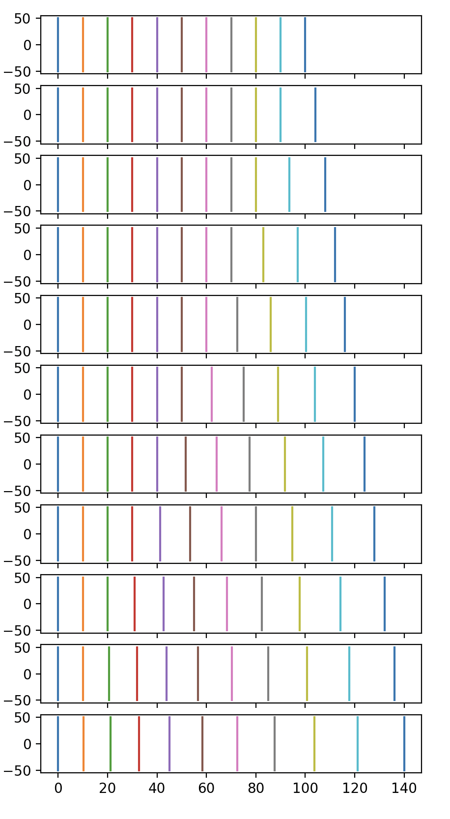
Here is the implementation of an approach that uses the speed of the pressure (rarefaction) wave through the spring, where the speed of the drawstring is 1/4 of the wave speed, set at 10 length units/time. I've used a spring with 11 coils, and an equilibrium length of 10 (arbitrary length units), and plotted the position of the coils over the 10 equal time intervals that coincide with the arrival of the pressure wave at that position on the spring. enter image description here

Here's the code:

('''
import matplotlib.pyplot as plt
import numpy as np
r = 50 #  length of the line
L0 = 100 # equilibrium length
N = 10 # number of segments
C = 10 # speed of propagation m/sec
V = 4. # speed of front coil m/sec
S = L0/N # segment length metres
TI = int(S)
L = np.zeros(C+1, dtype = float)
L[0] = L0  # lengths - metres
x = np.zeros((C+1, C+1),dtype = float)
#t=5 # coil number just starting to move, counting from rear
for n in range(TI+1): #time stamps
   wp = L0 - n*TI # wave position - moving back from the front of the spring
   if n >0:
       L[n] = L[0] + V*n # new length
       factor = L[n]  /(L[n-1])
   for c in range(N+1):  # segment number
       if n==0:# establish the first column (each coil, first time)
          x[c][n] = c*S
       elif x[c][n-1] <= wp : # wave not yet there
           x[c][n] = x[c][n-1]  # counting from rear of the coil, so up to wp the spring has not been disturbed.
       else :
           x[c][n] = x[c][n-1]*factor
# Create a figure with 11 subplots (1 row, 2 columns)
fig, axs = plt.subplots(11, 1, figsize=(5, 10),sharex=True)

# Plot on the first subplot
for i in range(N+1): 
   X = [x[:,i],x[:,i]]
   Y = [r, -r]
   axs[i].plot(X,Y)
plt.show() '''

`

This code generates the 11 position images: enter image description here

$\endgroup$

Your Answer

By clicking “Post Your Answer”, you agree to our terms of service and acknowledge you have read our privacy policy.

Not the answer you're looking for? Browse other questions tagged or ask your own question.