Compton Scattering Angle Distribution, and the Klein-Nishina Model

Question

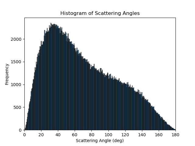
I have a Geant4 simulation where 662keV photons are going into a detecting volume (Germanium). As expected, when I look at the output of the simulation, these photons undergo Compton scattering and photoelectric absorption.

I have written a python script for analysing this output, where I calculate the scattering angle and plotted them in a histogram:

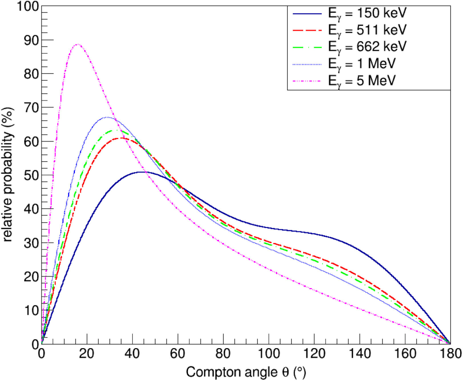
This seems to agree very well with plots I've found online. (figure2: DOI:10.1016/j.nima.2019.163228 )

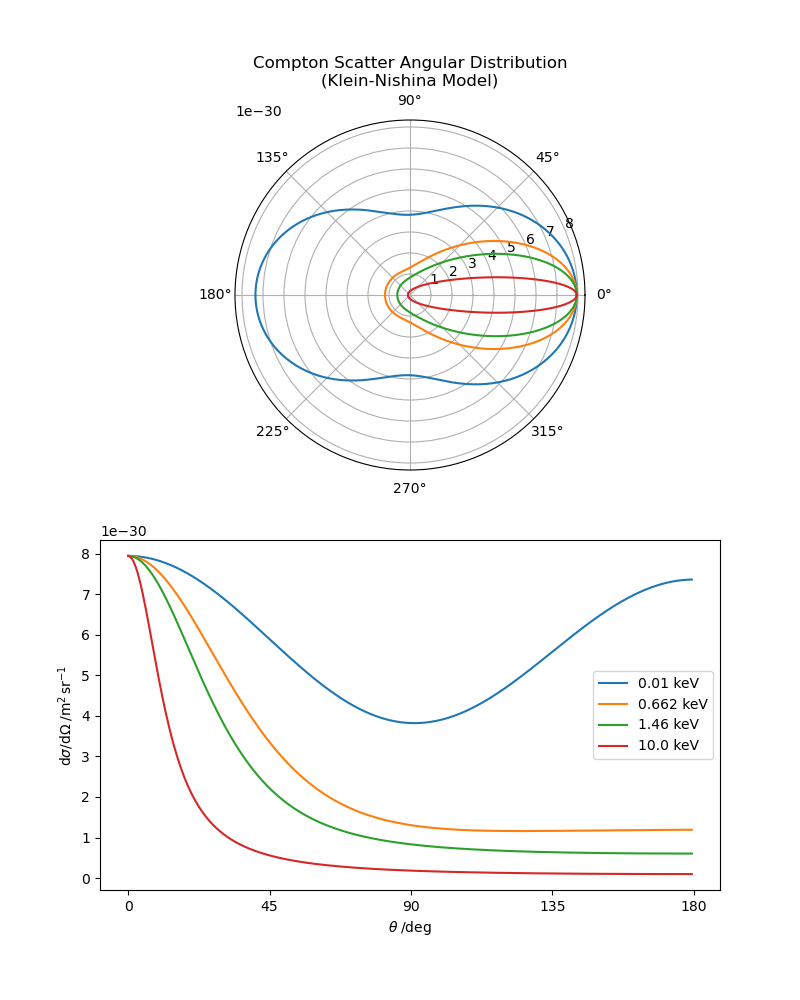
To round off this piece of work, I wanted to show that my distribution from Geant4 can be inferred from the Klein-Nishina model/the model that the aforementioned paper used.

However, when I plot the differential cross section (which I understood as akin to 'probability'?) vs scattering angle of the KN model, they don’t agree. The distribution shape is totally different.

The simulated electrons in the detecting volume aren't free electrons, so I tried adding an Impulse Approximation (Hartree-Fock if that means anything) but it still doesn't line up with the simulation results (although I'm not entirely sure if I did it right – the maths was slightly heavy for me).

How would I go about showing the agreement between theory (Klein-Nishina or other model) and my histogram?

And how did the author of the 'relative probability' graph obtain that data; a model that I don't know of, experimental...?

Any help or push in the right direction is hugely appreciated. :)

EDIT The answer below yields the below python script - although the vertical scale is off.

import numpy as np
import matplotlib.pyplot as plt

c = 299792458.0  # meter / second
E = 662000 *1.602176634 * 10**(-19) #incident energy 
h = 6.62607015 * 10**(-34)  # joule second
hbar = h / (2 * np.pi)
me = 9.1093837015 * 10**(-31)  # kilogram

omega = E / hbar #angular freq
R = hbar * omega / (me * c**2) #variable R in solution

def I(t):#define the function I(theta)
    return -np.cos(t) / R**2 + \
           np.log(1 + R * (1 - np.cos(t))) * (1/R - 2/R**2 - 2/R**3) - \
           1 / (2 * R * (1 + R * (1 - np.cos(t)))**2) + \
           1 / (1 + R * (1 - np.cos(t))) * (-2/R**2 - 1/R**3)

def w_prime(t):#Calc angular_freq for scattered photon
    return omega/(1+(hbar*omega/(me*c**2))*(1-np.cos(t)))

def f(t):#calc f(theta), aka the PDF
    return (1/(I(np.pi)-I(0))) * (w_prime(t)/omega)**2 * (omega/w_prime(t) + w_prime(t)/omega -(np.sin(t)**2))*np.sin(t)

theta_vals = np.linspace(0, np.pi, 1000)
f_vals=f(theta_vals)

plt.plot(theta_vals, f_vals)
plt.title("PDF")
plt.xlabel("Theta")
plt.ylabel("f(theta)")
plt.show()

Answer 1

$d\sigma$ needs to be converted to a probability density function $f(\theta)$, then plot $f(\theta)$.

The well-known cross section for Compton scattering is $$ \frac{d\sigma}{d\Omega} =\frac{\alpha^2(\hbar c)^2}{2s} \left(\frac{\omega'}{\omega}\right)^2 \left(\frac{\omega}{\omega'}+\frac{\omega'}{\omega}-\sin^2\theta\right) $$ where $$ \omega'=\frac{\omega}{1+\frac{\hbar\omega}{mc^2}(1-\cos\theta)} $$

We can integrate $d\sigma$ to obtain a cumulative distribution function. Let $I(\theta)$ be the following integral of $d\sigma$. (The $\sin\theta$ is due to $d\Omega=\sin\theta\,d\theta\,d\phi$) \begin{equation*} I(\theta)= \int \left(\frac{\omega'}{\omega}\right)^2 \left(\frac{\omega}{\omega'}+\frac{\omega'}{\omega}-\sin^2\theta\right) \sin\theta\,d\theta \end{equation*}

The solution is \begin{multline*} I(\theta)=-\frac{\cos\theta}{R^2} +\log\big(1+R(1-\cos\theta)\big)\left(\frac{1}{R}-\frac{2}{R^2}-\frac{2}{R^3}\right) \\ {}-\frac{1}{2R\big(1+R(1-\cos\theta)\big)^2} +\frac{1}{1+R(1-\cos\theta)}\left(-\frac{2}{R^2}-\frac{1}{R^3}\right) \end{multline*} where \begin{equation*} R=\frac{\hbar\omega}{mc^2} \end{equation*}

The cumulative distribution function is \begin{equation*} F(\theta)=\frac{I(\theta)-I(0)}{I(\pi)-I(0)}, \quad 0\le\theta\le\pi \end{equation*}

The probability of observing scattered photons in the interval $\theta_1$ to $\theta_2$ is \begin{equation*} P(\theta_1\le\theta\le\theta_2)=F(\theta_2)-F(\theta_1) \end{equation*}

Differentiate $F(\theta)$ to obtain normalized probability density function $f(\theta)$. $$ f(\theta)=\frac{dF(\theta)}{d\theta} =\frac{1}{I(\pi)-I(0)} \left(\frac{\omega'}{\omega}\right)^2 \left(\frac{\omega}{\omega'}+\frac{\omega'}{\omega}-\sin^2\theta\right) \sin\theta $$

Note that if we had carried through the $\alpha^2(\hbar c)^2/2s$ in $I(\theta)$, it would have canceled out in $F(\theta)$.