This is a very nice question, but to answer that, we should first clarify the OP in detail.
-- First scenario: Abrupt change
One may consider a scenario in which a ferromagnetic material prepared in an ordered state (eg., with $ \langle m \rangle = \uparrow $) is suddenly subjected to a finite “opposite” external magnetic field (ie., antiparallel to the initial magnetisation) while the temperature is kept fixed below the critical temperature.
I think this abrupt scenario cannot be called a phase transition in the common sense. Such a procedure will induce an abrupt change in the properties of the system (esp. its ground-state). Free energy will be discontinuous itself, so it is a “zeroth-order/discontinuous phase transition”, if you wish.
Phase transitions are usually defined as processes in which a slow variation of a thermodynamic variable (usually, temperature) leads to drastic changes in the thermodynamic phase of a system. Abrupt changes are trivial in this regard: we know a priori that they induce qualitative changes in the system. In our case, if one changes the external magnetic field abruptly, and waits long enough to let the system relax to its equilibrium, one will see that the magnetisation of the system is reversed to be parallel to the final external field; the system adapts itself to the applied field if we allow it to relax (see diagram below).
                               *************
                 apply H     ** complicated **
initial phase  ———————————>  **  relaxation **  ———>  final phase
                             **   process   **
                               *************
Notice that the devices of equilibrium statistical mechanics cannot deal with the intervening inherently non-equilibrium relaxation process. They can only explain the equilibrium initial and final (ordered) phases. In our scenario, we implicitly assume that we wait long enough for the system to relax.
So let's consider a quasi-static (slow) scenario. But, to be more quantitative, we need a simple mean-field analysis.
-- Mean-field analysis
To consider the transition more quantitatively, let's model a ferromagnetic material with a nearest-neighbour Ising model ($ S = \frac{1}{2} $), and “solve” it within the mean-field approximation. The derivations of the mean-field Hamiltonian and partition function are given in modern statistical physics textbooks and will not be repeated here (see eg., Schwabl, F. “Statistical Mechanics” (2010) [WCat]).
The dimensionless mean-field free energy density reads
$$
f(h, T; m) := \frac{1}{T_c} \frac{F}{N} = \frac{1}{2} m^2 - \frac{T}{T_c} \ln \big( 2\cosh( \mathcal{M}_h ) \big)
$$
where $ \mathcal{M}_h := \frac{T_c}{T} ( h + m ) $, $ h $ is the rescaled external magnetic field, $ h := h_{ext}/T_c $, $ m $ is the mean-field, $ T_c $ is the critical temperature for spontaneous magnetisation, and $ T $ is the temperature. Note that we use natural units where $ k_B = 1 = \hbar $.
To determine the mean-field $ m $, we minimize the free energy and obtain the self-consistent mean-field equation,
$$
m = \tanh( \mathcal{M}_h ) ~.
$$
The nature of the solutions for $ T < T_c $ differs from those for $ T > T_c $: ie., in absence of external fields, $ h \rightarrow 0 $, we have a finite spontaneous magnetisation ($ m \neq 0 $) when $ T < T_c $, but no spontaneous magnetisation ($ m = 0 $) when $ T > T_c $.
From the free energy, one can readily obtain the entropy,
$$
s := \frac{S}{N} = - \frac{1}{N} \frac{\partial F}{\partial T} \big\vert_{V, h}
= \ln \big( 2 \cosh(\mathcal{M}_h) \big) - m \, \mathcal{M}_h ~,
$$
specific heat at constant volume, $ c_V $,
$$
c_V := \frac{C_V}{N} = \frac{1}{N} T \frac{\partial S}{\partial T} \Big\vert_{V, h} = -\frac{1}{N} T \frac{\partial^2 F}{\partial T^2} \Big\vert_V
= - \frac{T \mathcal{M}_h^2}{1 - \frac{T}{1 - m^2}} ~.
$$
and magnetic susceptibility, $ \chi_h $,
$$
\chi_h := \frac{\partial m}{\partial h} = - \frac{1}{1 - \frac{T}{1 - m^2}} ~.
$$
To obtain the relations above, we have used a rescaled temperature, $ T \mapsto \frac{T}{T_c} $, and plugged in the mean-field equation and its temperature derivative,
$$
\frac{\partial m}{\partial T} = \frac{\mathcal{M}_h}{1 - \frac{T}{1 - m^2}} ~,
$$
when necessary.
According to the Ehrenfest classification (see this figure), the order of a transition can be determined from the discontinuities in the derivatives of the free energy (see Side Remarks).
-- Second scenario: Quasi-static change
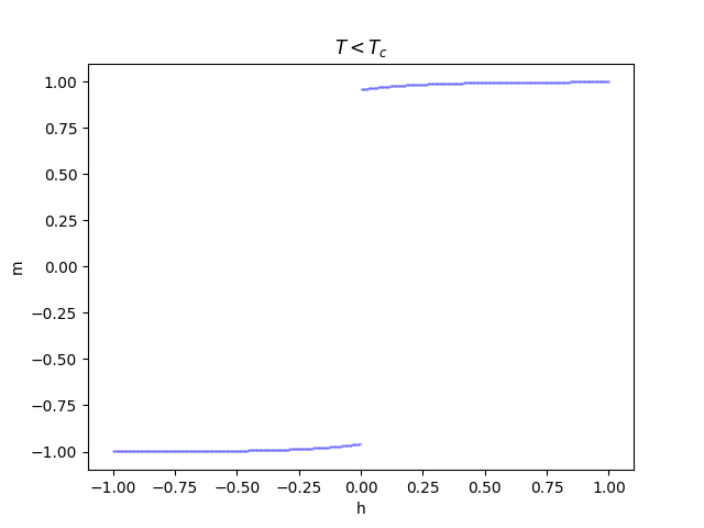
One may consider a variation of the first scenario where, at a fixed $ T < T_c $, the strength of the magnetic field is slowly (quasi-statically) varied from a positive value to some negative value. We observe that in this case, $ m $ has a jump at $ h = 0 $ (see figure below); therefore, a discontinuous (1st-order) phase transition happens when $ h $ crosses 0.

For concreteness, let's suppose that we prepare the system in a preferred magnetised state (say, $ \uparrow $) with a tiny external field $ h_\uparrow $ in a temperature $ T < T_c $, and then we slowly vary the magnitude of the field to a finite value $ h_\downarrow $ in the opposite direction. Then we calculate the free energy and entropy in the initial and final phases and changes thereof:
$$
\Delta f := f(h_\downarrow, T) - f(h_\uparrow, T) \\
\Delta s := s(h_\downarrow, T) - s(h_\uparrow, T) ~;
$$
from this we obtain the exchanged heat in the process,
$$
\Delta q = T \Delta s ~.
$$
First order phase transitions are always associated with a latent heat?
If the initial and final applied fields have the same magnetisation, since the entropy is an even function of $m$, then there will be no entropy change and hence, no heat exchange, $ \Delta q = 0 $, as mentioned by OP.
Here, it is important to note the presumptions behind statements like “first-order phase transitions are associated with a latent heat”. The measurement scenario presumed for this statement is that one varies the temperature quasi-statically and measures the thermodynamic quantities as temperature crosses a certain value $ T_\ast $. In the case of a “first-order transition”, varying the temperature across $ T_\ast $ will incur a finite latent heat. Thus, that is not a statement about arbitrary external fields, like magnetisation. However, there is still an analogy.
In our scenario, when the magnetic field is changed slowly from $ h_\ast - \delta h $ to $ h_\ast + \delta h $, with a small $ \delta h > 0 $, then the internal energy of the system suddenly changes by a finite value $ \sim m \, \delta h + h_\ast \, \delta M $, due to the discontinuity of $ m $ at $ h_\ast $. This amount of energy is absorbed from/released to the external field -- this is essentially the work performed by the external field on the system which leads to a change in the internal energy as $ du = đ q + dw $. This is similar to the usual case when temperature is varied near the transition point and a latent heat $ \Delta q $ is absorbed from/released to the reservoir.
-- Side Remarks
(I) Is this scenario truly a first-order phase transition?
The fact that this scenario is indeed a first-order phase transition, can be seen by an analysis of singularities in thermodynamic quantities. First let's consider the magnetisation. The mean-field equation can be expanded around $ h = 0 $ in an ordered phase where $ \frac{T}{T_c} \lesssim 1 $ and $ m \sim \mathcal{O}(1) $ is finite. Then we obtain the approximate mean-field equation,
$$
m \sim \tanh(m/T) + \frac{h}{T} ( 1 - \tanh^2(m/T) ) ,
$$
where only the leading linear term in $ h $ is kept (“linear response” approximation).
Since $ m $ and $ T $ are $ \mathcal{O}(1) $, we can replace the $\tanh$ functions with their asymptotic values; namely,
$$
\tanh(m/T) \sim \text{sign}(m) \sim \text{sign}(h) = \pm 1 ~;
$$
The second approximation is valid since the sign of $ h $ determines the sign of $ m $ (see above). From this, we readily get the non-analyticity in $ m(h) $ near $ h = 0 $ (in the ordered phase when $ T < T_c $):
$$
m \sim \text{sign}(h) ~.
$$
By an analogous method, we can see that entropy has also a singularity:
$$
s = - \frac{\partial f}{\partial T} \sim \text{const.} - \frac{h}{T} (m \, \frac{\partial m}{\partial h}) ~.
$$
The derivative, $ \frac{\partial m}{\partial h} $ behaves like a $\delta$-function, so we can “model” it by a Lorentzian of infinitesimal width $\varepsilon$,
$$
\frac{\partial m}{\partial h} = \lim_{\varepsilon \rightarrow 0} \frac{1}{h^2 + \varepsilon^2} ~,
$$
where unnecessary factors are dropped in the Lorentzian. Then, the entropy behaves as
$$
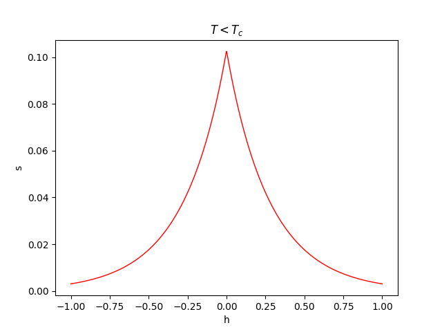
s \sim \lim_{\varepsilon \rightarrow 0} \frac{h \, \text{sign}(h)}{h^2 + \varepsilon^2} = \lim_{\varepsilon \rightarrow 0} \frac{| h |}{h^2 + \varepsilon^2} = - \frac{1}{|h|} ~.
$$
So, $ s(h) $ behaves non-analytically as $ -\frac{1}{|h|} $ in the vicinity of $ h = 0 $ (in the ordered phase when $ T < T_c $) (see figure below). This completes the picture of the discontinuous phase transition.

(II) The Python code to compute and visualize all of these is accessible here.


