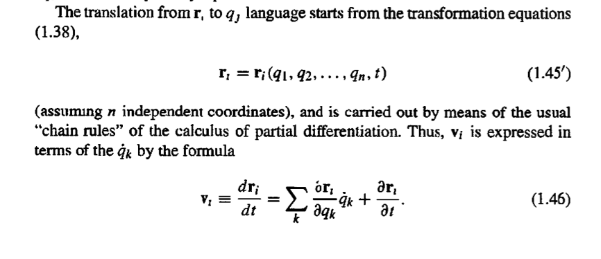
In these notes,
$\frac{\partial \vec{r}} {\partial q_i}$ is stated to form a basis set for the vector space. How does this happen?
Also, how does one justify this equation from Goldstein's Classical Mechanics using the above method?

In these notes,
$\frac{\partial \vec{r}} {\partial q_i}$ is stated to form a basis set for the vector space. How does this happen?
Also, how does one justify this equation from Goldstein's Classical Mechanics using the above method?

Consider a system made of $N$ points of matter, with positions $\vec{r}_i$, $i=1,\ldots,N$ referred to the rest space of a reference frame $\cal I$. In the absence of further constraints, the system is described in $\mathbb R^{3N+1}$, where $\mathbb R^{3N}$ refers to the spatial Cartesian coordinates of the points in $\cal I$, whereas the last $\mathbb R$ indicates the axis of time $t$.
Next, suppose that the points are assumed to satisfy some constraints described by $c < 3N$ conditions, $$f_j(t,\vec{r}_1,\ldots, \vec{r}_N) =0\quad j=1,\ldots, c\:.\tag{1}$$ For instance the conditions above may state that some distances between $\vec{r}_i$ and $\vec{r}_j$ is a given function of time, or that some of the points belong to lines or surfaces fixed in $\cal I$, or deforming in time with a given law (a circumference with radius $R(t)$ depending on time), and so on. Assume that the functions $f_j$ are smooth ($C^2$ would be enough) and focus on the Jacobian matrix of elements $$\frac{\partial f_j}{\partial x_{ik}}$$ where $\vec{r}_i = x_{i1}\vec{e}_1+ x_{i2}\vec{e}_2+ x_{i3}\vec{e}_3$. If that matrix has $c$ linearly independent row (or culumn) on the set $S \subset \mathbb R^{3N+1}$ defined by (1), the constraints are said holonomic.
In this case as a straightforward consequence of the so called theorem of regular values it is possible to prove that, every $a\in S$ admits a neighbourhood $U_a$, such that $S \cap U_a$ is biunivocally and smoothly described by local coordinates $t, q_1,\ldots, q_n$ with $n= 3N-c$ and where $t$ is the initially used time coordinate.
In other, more mathematical, words $S$ is an embedded submanifold of $\mathbb R^{3N+1}$ and $t, q_1,\ldots, q_n$ are a local coordinate system.
For every fixed $t_0$, the elements $a$ of $S$ with $t(a)=t_0$ define the configuration space of the system at $t=t_0$. That is an emebedded submanifold of $S$ (and thus of $\mathbb R^{3N+1}$) with dimension $n$.
REMARK. It is possible to prove (using again the mentioned theorem) that the $n$ coordinates $q_k$ can always be chosen to coincide with $n$ of the components $x_{ij}$. The remaining coordinates are functions of $t$ and the $q_k$ through functions of the same regularity ($C^2$ in our case) as that of the functions $f_j$.
Since $t,q_1,\ldots, q_n$ are free coordinates to describe the system, we can write down $N$ vector valued $C^2$ functions: $${\vec r}_i= {\vec r}_i(t,q_1,\ldots,q_n)\quad i=1,\ldots, N \tag{2}$$ It is not so difficult to prove that, in view of the above remark, the vectors $$\frac{\partial \vec{r}_i}{\partial q_k}$$ must be linearly independent. They form a basis of the tangent space at each point of the submanifold $S_t$.
The coordinates $q_1,\ldots, q_n$ are the ones used to describe the motion of the system. Each motion is defined by a curve $\mathbb R \ni t \mapsto (q_1(t),\ldots, q_n(t))$. Motion in physical space is then obtained just exploiting (2), $$\mathbb R \ni t \mapsto \vec{r}_i(t, q_1(t),\ldots, q_n(t))\:,\quad i=1, \ldots, N \tag{3}\:.$$ Looking at (3), it is should be obvious that the velocity of the point determined by $\vec{r}_i$ with respect to $\cal I$ is given by $$\vec{v}_i(t) = \frac{d\vec{r}_i}{dt} = \frac{\partial \vec{r}_i}{\partial t} +\sum_{k=1}^n \frac{\partial \vec{r}_i}{\partial q_k} \dot{q}_k\quad\mbox{with}\quad \dot{q}_k := \frac{dq_k}{dt}\:.$$