2
$\begingroup$

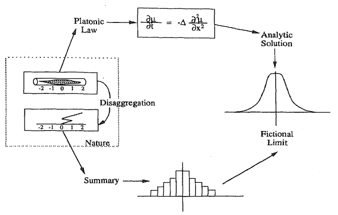
Peter Galison "Computer Simulations and the Trading Zone", page 147

In the above diagram, the author (Peter Galison) describes the capillary-tube diffusion process (in "Computer Simulations and the Trading Zone") as modeled by a partial differential equation (top), and then as imitated by a Monte Carlo simulation of a stochastic process of, for example, flipping a coin and moving to the right when a head falls and to the left when a tail falls (bottom).

I've been struggling to understand how Monte Carlo simulations are used in physics. The author describes Monte Carlo simulation as an alternative to solving the partial differential equation. In this example of a Monte Carlo simulation for the capillary-tube diffusion process it is not clear to me what is known and what is unknown/sought to be discovered by the simulation:

  1. The goal of the simulation as I understand it is to approximate the pictured the bell-shaped distribution obtained by analytic solution. What is on the x-axis in the bell shaped curve?
  2. The author says that the simulation could be done by "flipping a coin and moving to the right when a head falls and to the left when a tail falls". Are we talking about a fair coin so that P(Heads)=P(Tails). By how much will we move to the right or to the left in each instance?

Big picture, I don't understand how we would build a Monte Carlo simulation and use it to learn something about a process, such the one above. What is assumed to be known? What is unknown? Obviously if I took a fair coin and decided to move to the right by 1 unit if the coin turns up Heads and move to the left by 2 units if the coin turns up Tails, 1) we would not learn anything useful from this model and 2) this model would have nothing to do with the capillary-tube diffusion process. How then do we build such a model?

$\endgroup$
1
  • 2
    $\begingroup$ monte carlo simulation is used when there are multiple risk factors and multiple steps involved such that it is too complicated or troublesome to find the analytical probability destribution of the final outcome. In late game monopoly, for eg, it might be hard to form a full probability analysis of you making a full round without going bankrupt. many steps are involved, each step has a random die-based outcome, there may be choices to buy or not to buy land when landing on certain spots, etc. Doing many simulations grant a survey of possible outcomes, which may help in risky decision making. $\endgroup$
    – James
    Commented Nov 26, 2022 at 14:30

1 Answer 1

4
$\begingroup$

Diffusion processes can be easily interpreted with a probabilistic approach.

1D diffusion process - probabilistic approach. Let's divide the space and time in a discrete set of points and time intervals, with points of coordinates $x_n = n \Delta x$, and time instants $t_i = i \Delta t$.

Now, let's consider the probability of state transition from state $x_n$ at time instant $t_i$ to the states $x_k$ at time instant $t_{i+1}$, and let's define the probability transition as

$T(x_k,t_{i+1}; x_n, t_i) = \left\{ \begin{array} \\ d \qquad \qquad , x_k = x_{n-1} \\ 1-2d \qquad , x_k = x_{n} \\ d \qquad \qquad , x_k = x_{n+1} \\ 0 \qquad \qquad , \text{otherwise} \end{array} \right. $,

i.e. starting from $x_n$, the probability of being in state $x_{n}$ at the next time-step is $1-2d$, the probability of being in neighboring states $x_{n\pm1}$ is $d \ge 0$, and it's zero for all the other states.

Thus the overall probability of being in state $x_n$ at time $t_{i+1}$ is equal to

$p(x_n, t_{i+1}) = (1-2d) p(x_n, t_i) + d p(x_{n-1}, t_i) + d p(x_{n+1}, t_i)$,

that can be rearranged as

$p(x_n, t_{i+1}) - p(x_n, t_i) = d p(x_{n-1}, t_i) -2d p(x_n, t_i) + d p(x_{n+1}, t_i)$.

The left-hand side could be interpreted as a first-order discrete approximation of the time derivative (using explicit Euler method),

$p(x_n, t_{i+1}) - p(x_n, t_i) = \Delta t \dfrac{\partial p}{\partial t}(x_n, t_i) + o(\Delta t) $

and the right-hand side could be interpreted as a discrete approximation of the second-order space derivative

$p(x_{n-1}, t_{i}) - 2p(x_{n}, t_i) + p(x_{n+1}, t_i) = \Delta x^2 \dfrac{\partial^2 p}{\partial x^2}(x_n, t_i) + o(\Delta x^2) $,

and thus, we can rearrange the probability equation as

$ \Delta t \dfrac{\partial p}{\partial t}(x_n, t_i) + o(\Delta t) = d \Delta x^2 \dfrac{\partial^2 p}{\partial x^2}(x_n, t_i) + o(\Delta x^2)$,

and letting $\Delta x \rightarrow 0$, $\Delta t \rightarrow 0$, so that $d \frac{\Delta x^2}{\Delta t} = D$ finite,

$\dfrac{\partial p}{\partial t}(x, t) = D \dfrac{\partial^2 p}{\partial x^2}(x, t)$.

Montecarlo simulation.

  • I'd use a finite volume, or a finite difference method;

  • dividing the space domain in cells of size $\Delta x$, and using time-step $\Delta t$, so that the diffusivity $D$ and the probability $d$ are related by $D = \frac{d \Delta x^2}{\Delta t}$;

  • You can initialize a vector of:

    • the dimension of the number of the particles you're using to represent the concentration of your specie

    • collecting the id of the cell where you find the particles.

      $\mathbf{u}_i = \left[ u^1_i, u^2_i, u^3_i, \dots u^N_i \right]$

      so that the concentration in the cell $x_n$ is the number of particles of in each cell divided by the cell volume, and thus it's proportional to the number of elements of $\mathbf{u}$ equal to $x_i$, $\rho(x_n) \sim N(u^k = x_n)$.

  • apply transition probability $T(x_k, t_{i+1}, x_n, t_i)$, using a random or a pseudorandom number generator, to get $\mathbf{u}_{i+i}$.

Python implementation - Colab. Here, I'm attaching a Colab sheet with the implementation of the method. This is in Python, and with unnecessary for loops. Even though it's not the most efficient implementation, it should be a working one.

https://colab.research.google.com/drive/1l12iIilelFFygJFIjkdAitY1ZXwFCrvy?authuser=3#scrollTo=azhJykNbROCV

Here,

  • 1000 particles sampled from uniform distribution in the range $x \in [0, 1]$
  • infinite domain,
  • pay attention at the Courant-Friedrichs-Lewy (CFL) condition, that relates $D$, $\Delta x$, to the $\Delta t$ to get $d \le 0.5$, and thus probability $\in [0,1]$ in transition matrix $T$.
$\endgroup$
9
  • 1
    $\begingroup$ +1: Thank you. The link to the code didn't work for me, unfortunately. I'll try again. $\endgroup$ Commented Nov 26, 2022 at 15:26
  • $\begingroup$ I forgot to make the GIST. Try this one gist.github.com/Dade1989/a564620475b40d7594c587bdf19fea5c. Open in Colab and run $\endgroup$
    – basics
    Commented Nov 26, 2022 at 15:36
  • 1
    $\begingroup$ Note that we understand diffusion models based on differential equations as approximations of more realistic probabilistic models of the microscopic physics. So, it's not too surprising that you may return to a probabilistic model (on a different scale to be practical). $\endgroup$
    – John Doty
    Commented Nov 26, 2022 at 15:59
  • 1
    $\begingroup$ This is very insightful. I should have mentioned that my background is economics so I might be confused about things that are taken for granted in physics, in a diffusion problem. To save myself such potential confusion, can you please describe what is plotted on the x-axis in the final density plot that your problem produces? Thank you in advance. $\endgroup$ Commented Nov 26, 2022 at 16:49
  • 1
    $\begingroup$ gist.github.com/Dade1989/4ad40749926cfa47d1dbb947d06f621a updated gist, with a plot in the the for loop, so that you can see the evolution of the system $\endgroup$
    – basics
    Commented Nov 26, 2022 at 17:27

Your Answer

By clicking “Post Your Answer”, you agree to our terms of service and acknowledge you have read our privacy policy.

Not the answer you're looking for? Browse other questions tagged or ask your own question.