In Goldstein problem 3.5, We have to calculate the scattering angle, $\Phi(s)$, given as a function of input parameter, using Gauss-Legendre Quadrature. The full question is as follows;
Compute numerically $\Phi(s)$ and the differential cross section of $\sigma(\Phi)$ for the repulsive potential $$V=\frac{V_0}{1+r}$$ and for total energy $E=1.2V_0$. It is suggested that the 16-point Gauss-Legendre quadrature will give adequate accuracy. Does the scattering exhibit a rainbow?
So firstly starting with $\Phi(s)$ given as: $$\Phi(s)=\pi-2\displaystyle\int_{r_m}^\infty\frac{sdr}{r\sqrt{r^2 \left(1-\frac{V(r)}{E}\right)^2 - s^2}} \tag{1}$$
Where $s$, is the impact parameter. $r_m$ is the radius at closest approach and $r$ is the radius from the centre of the force. Defining some function $\rho(r)=\sqrt{1-\frac{r_m}{r}}$ and inserting into $(1)$ we get the scattering angle as
$$\Phi(s) = \pi-4s \displaystyle\int _0^1 \displaystyle\dfrac{\rho \ d \rho}{\sqrt{r_m^2(1-\frac{V}{E})^2-s^2(1-\rho^2)^2}} \tag{2}$$
the formulation of the scattering angle in equation $(2)$ allows us to use Gauss-Legendre quadrature mainly because of the definite limits of integration and the fact that the integrand is non singular in between those limits.
So I created a Gauss-Legendre quadrature algorithm in python
import sympy
from sympy import legendre, real_roots, nroots, diff
import numpy as np
import matplotlib.pyplot as plt


def weights_and_roots(p):
    '''
    calculates the roots of a P+1 degree Legendre polynomial then uses them to calculate the weights
    '''
    c = []
    L = legendre((p+1),x)
    dL = L.diff(x)
    nR = nroots(L)
    for rt in nR:
        c.append(2/((1-rt**2)*dL.evalf(subs={x:rt})**2))
    return c, nR

def GLI(c,nR,f,lower_limit=-1,upper_limit=1):
    '''
    c = list of all the weights calculated in the previous function
    nR = this is a list of all the roots again calculated in the previous function
    f = the function being numerically integrated
    lower_limit = the lower limit of integration
    Upper_limit = the upper limit of integration

    The following sums the weights with the function (f) evaluated at the respective legendre root
    '''
    idx = len(nR)
    S = 0
    for i in range(idx):
        S+= ((upper_limit-lower_limit)/2)*c[i]*f.subs(x,(((upper_limit-lower_limit)/2)*nR[i]+((upper_limit+lower_limit)/2)))
    return S
I tested it on some known functions and it worked well so I tried applying it to the integral in equation $(2)$ with $V$ as given in the question, I also replaced the $r_m^2$ with $r(1-\rho^2)^2$ thus the integral in equation $(2)$ is given as
$$\displaystyle\int _0^1 \displaystyle\dfrac{\rho \ d \rho}{\sqrt{(r(1-\rho^2)^2(1-\frac{1}{1.2(1+r)})^2-s^2(1-\rho^2)^2}} \tag{3}$$
My reasoning for replacing $r_m^2$ is because we don't know this value before hand so just sticking a value in felt wrong. I then ran equation $(3)$ through my Gauss-Legendre quadrature code. I set $r$ as $20$ and I set $V_0$ as $10$ as well just to give them values. The code is as follows
r = sympy.Symbol("r") #radius
s = sympy.Symbol("s") # impact parameter
x = sympy.Symbol("x") # I use x instead of rho

a = 20 #setting the radius

f = x/((((r*(1-x**2))**2)*(1-(1/1.2*(1+r)))**2)-(s*(1-x**2))**2)**(1/2)
p =16 # number of points

c,nR = weights_and_roots(p)
S = GLI(c,nR,f,0,1)
print(S)

phi = np.pi - 4*s*S #Calculate Phi
phi = phi.subs(r,a) # substitute a value for the radius r given by a
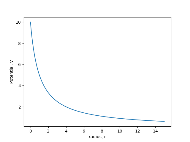
Plotting the potential as a function of radius gave the following Graph
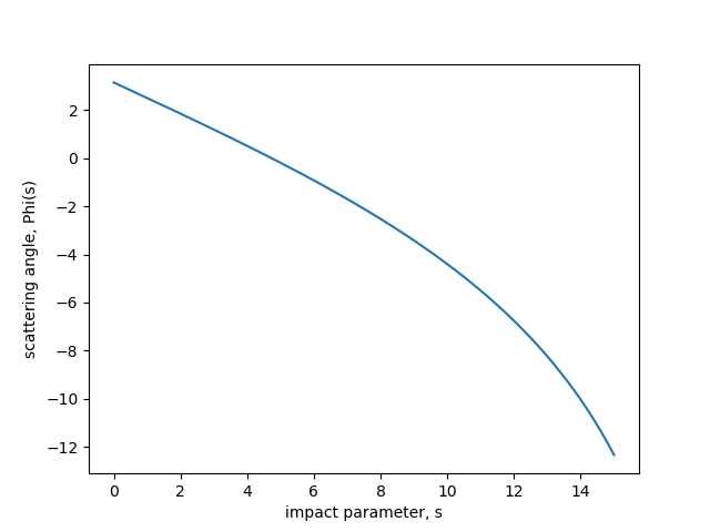
However, when I plotted $\Phi(s)$ calculated using the script shown above as a function of impact parameter, $s$. I got the following graph
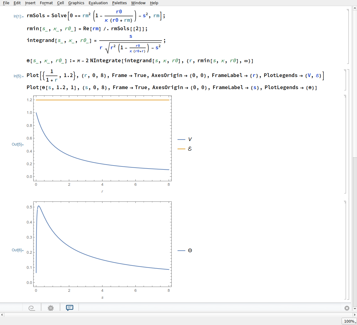
However, this doesn't look right to me at all! I would assume the scattering angle to fall away to zero as the impact parameter increases. However I am not sure where I have gone wrong? Furthermore, the question askes if the scattering exhibits a rainbow but I am not sure what sort of scattering profile is evidence of a rainbow scattering effect.


