0
$\begingroup$

I want to very simplistically plot the $x$-$y$ position of a vehicle in 2D that can accelerate/brake and drive a constant speed while turning etc.

The basic equations for determining the position for constant speed seem to be

$$x_{n+1} = x_n + vt\cos(\theta)$$ $$y_{n+1} = y_n + vt\sin(\theta)$$

where $\theta$ is the turning angle given in radians.

Am I correct in assuming that since $$v_{n+1} = v_n + at$$ for a constant acceleration we have:

$$x_{n+1} = x_n + (v_n+at)t\cos(\theta)$$ $$y_{n+1} = y_n + (v_n+at)t\sin(\theta)$$ ?

$\endgroup$
7
  • $\begingroup$ This does not allow to turn, since the acceleration is always the same for both components! $\endgroup$ Commented Dec 21, 2020 at 12:38
  • $\begingroup$ Hello @AlmostClueless would you mind suggesting an alternative formula ? Thanks ! $\endgroup$
    – Tony_V
    Commented Dec 21, 2020 at 12:44
  • $\begingroup$ You are missing a factor 1/2 and you should allow for $a_x \ne a_y$. $\endgroup$
    – NotMe
    Commented Dec 21, 2020 at 13:05
  • $\begingroup$ Hello @Semoi , the factor $\frac{1}{2}$ should be added at $\frac{1}{2}at$ ? Does this fix the issue pointed out by AlmostClueless ? Would you mind directing me perhaps at some resources that could help someone fix this problem without much physics knowledge ? $\endgroup$
    – Tony_V
    Commented Dec 21, 2020 at 14:45
  • $\begingroup$ A good point to start is probably google and "wiki acceleration position pdf". There are hundred of thousand links describing this relationship. Thus, the only problem is to find something, which is at your level. I reckon this is a problem, which is unavoidable $\endgroup$
    – NotMe
    Commented Dec 21, 2020 at 16:46

3 Answers 3

0
$\begingroup$

So I did a little C# demo to check that my math is correct first.
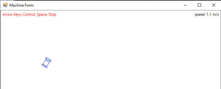
fig1

The math behind each simulation step is as follows (assuming non-zero steering angle). Below $\Delta t$ is the time step, $v_0$ the initial speed, $\vec{p}_0$ is the initial position, $\varphi_0$ the initial orientation angle, and $\ell$ is the wheelbase.

  1. Define the step steering angle $\theta$, as well as the acceleration $\dot{v}$.
  2. Define the turn radius $R = \ell / \tan \theta$.
  3. Get speed change $\Delta v = \dot{v} \Delta t$.
  4. Get distance change $\Delta s = v_0 \Delta t + \tfrac{1}{2} \dot{v} \Delta t^2$.
  5. Get orientation angle change $\Delta \varphi = \Delta s / R$
  6. Get new orientation angle $\varphi_1 = \varphi_0 + \Delta \varphi$
  7. Get initial normal direction $\hat{n}_0 = \pmatrix{-\sin (\varphi_0) & \cos (\varphi_0)}$
  8. Get final normal direction $\hat{n}_1 = \pmatrix{-\sin (\varphi_1) & \cos (\varphi_1)}$
  9. Get position change $\Delta \vec{p} = R\, (\hat{n}_0 - \hat{n}_1)$
  10. New position $\vec{p}_1 = \vec{p}_0 + \Delta \vec{p}$
  11. New speed $v_1 = v_0 + \Delta v$
  12. Get tangent direction $\hat{e}_1 = \pmatrix{ \cos(\varphi_1) & \sin(\varphi_1)}$
  13. Get new velocity vector $\vec{v}_1 = v_1 \hat{e}_1$

NOTE: All angles are in radians. The car position is defined by the center of the rear axle since a car turns about the rear wheels.

The key to this and the answer to your question is #9. It takes the current position, moves to the center of rotation (pivot point), and back into the new position by traversing an arc of length $\Delta s$.


The kinematics of a 2D car is described by the following picture
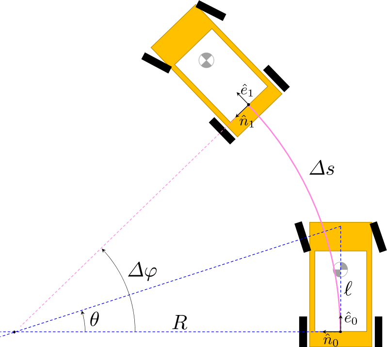
fig2

where $R$ is the radius of turn (and $1/R$ is the turn curvature). In pink is the arc the car tracks (the local coordinate of the car shown mid-rear axle) and it has an arc length of $\Delta s$. This arc sweeps an angle of $\Delta \varphi = \Delta s/R$. The angle $\theta$ describing the big blue triangle is the steering angle, due to similar triangles in the steering geometry.

The initial and final position and orientation of the car coordinate system is shown at the ends of the pink arc, and you see they share the common pivot point which is always $R$ distance away, along the $\hat{n}$ direction.

$\endgroup$
5
  • $\begingroup$ This is brilliant ! Thank you so much ! Would you mind sharing your code ? $\endgroup$
    – Tony_V
    Commented Dec 24, 2020 at 4:50
  • $\begingroup$ @Tony_V - github.com/ja72/CarControlForm $\endgroup$ Commented Dec 24, 2020 at 15:31
  • $\begingroup$ @Tony_V - I added a sketch to describe the quantities a bit better $\endgroup$ Commented Dec 24, 2020 at 15:57
  • $\begingroup$ Jesus Christ man this is just super. Thank you so much for the effort ! $\endgroup$
    – Tony_V
    Commented Dec 25, 2020 at 1:18
  • $\begingroup$ @Tony_V - thank you for your kind words. This kind of stuff is easy for me, no effort really. I have been doing mechanical simulations all my life. Glad I could help. $\endgroup$ Commented Dec 25, 2020 at 4:14
0
$\begingroup$

Your ($v_n$ + at) is a final velocity. With constant acceleration, you can divide that by two to get the average velocity. In general, with constant acceleration: x = $x_o$ + $v_{ox}$t + (1/2)${(a_x)(t^2})$ There would be a similar equation for y (or z).

$\endgroup$
0
$\begingroup$

There are two cases I will address. In your question, you say "constant acceleration", which is trivial to model since you only need to plug the kinematic equations into your software and plot with known values. The next is non-constant acceleration, which needs a numerical solution.

The simplest numerical model for this would be Newton's Method. Essentially we discretize the coordinates (since computers can only approximate continuous systems). Hence \begin{equation} \frac{d\vec{v}}{dt} = \vec{a}(t) \rightarrow \vec{v}_{n+1} = \vec{v}_{n} + \vec{a}_{n}\Delta t \end{equation} And to go from velocity to position \begin{equation} \vec{r}_{n+1} = \vec{r}_{n} + \vec{v}_n\Delta t \end{equation} Each of these vector equations are really two one-dimensional equations (assuming the equations are not coupled, which could still be solved numerically) in both the $x$ and $y$ directions. For example, \begin{equation} x_{n+1} = x_{n} + v_{x,n}\Delta t \end{equation} You can now take these equations and plug it into any software (python, mathematica; probably not a calculator though) and specify the acceleration (for both the $x$ and $y$ directions), how big you want the time steps, and how many time steps you want to take. Then let your computer step the system forward in time with the equations above, save that data to a list or array, and plot the position against time.

$\endgroup$
1
  • $\begingroup$ Thank you very much for providing me with the info on non constant acceleration @Richard Whitehill $\endgroup$
    – Tony_V
    Commented Dec 22, 2020 at 12:07

Your Answer

By clicking “Post Your Answer”, you agree to our terms of service and acknowledge you have read our privacy policy.

Not the answer you're looking for? Browse other questions tagged or ask your own question.