A discrete time Ornstein-Uhlenbeck type process

Question

Let's consider a stochastic process $$X_{t+1}=X_{t}+\Delta X_t$$ where $\Delta X_t$ is a Gaussian with mean $-\lambda X_t \Delta t$ and variance $2\Delta t$ where $\lambda$ and $\Delta t$ are parameters of the model.

We can then write the transition probability density as \begin{equation} P(X_{t+1}=x|X_{t}=y)=\frac{1}{\sqrt{4\pi\Delta t}}\exp\left[\frac{[x-y(1-\lambda \Delta t)]^2}{4\Delta t}\right] \end{equation}

We can find the stationary distribution of this process which will take the form \begin{equation} P_{\infty}(x)=\sqrt{\frac{a}{2\pi}}e^{-ax^2/2} \end{equation} where $a$ depends on the parameters $\lambda$ and $\Delta t$. It is easy to see that if we scale time by $\Delta t$ and in the limit $\Delta t$ goes to $0$, we get something like the Ornstein-Uhlenbeck process.

If we initialise the process in state $X_0$ distributed as the stationary state, and then want the $t$-step propagator of this process, which is, $P(X_t=x|X_0=0)$, it is easy to see that this will also be a Gaussian (as it is a sum of Gaussians). But is there a way to compute the distribution exactly?

Answer 1

So you could start with the propagator, chain them together and integrate over the intermediate values and you'll end with a discretized version of the path integral. This is, however, rather tedious, so let's just instead write the stochastic difference equation: $$\Delta X_n = -\lambda \Delta t + \sqrt{2} \Delta W_n$$ Here $\Delta W_n$ are independent Gaussian increments with variance $\Delta t$ and mean $0$; $W_0 = 0$. Note then that $\sum_{n=0}^{N-1} \Delta W_n = W_N - W_0 = W_N \sim \mathcal{N}(0, \Delta t N)$ as variance is additive. So I guess you can see where we're going with this: $$X_N - X_0 = \sum_{n=0}^{N-1} \Delta X_n = \sum_{n=0}^{N-1} (-\lambda \Delta t + \sqrt{2} \Delta W_n) = -\lambda \Delta t N + \sqrt{2} W_N$$ So $X_N$ is normally distributed with mean $X_0 -\lambda \Delta t N$ and variance $2\Delta t N$.

Now none of this is related to Orstein--Uhlenbeck. Maybe instead you meant to say: $$\Delta X_n = -\lambda X_n \Delta t + \sqrt{2} \Delta W_n$$ This, like the above, can be solved much like the corresponding SDE. Start by the simpler: $\Delta Z_n = -\lambda Z_n \Delta t \Rightarrow Z_{n+1} = (1-\lambda \Delta t) Z_n \Rightarrow Z_n = (1-\lambda \Delta t)^n Z_0$, and so we make the substitution $X_n = (1-\lambda \Delta t)^n Y_n$ to the original equation and are left with: $$(1-\lambda \Delta t)^{n+1}Y_{n+1} - (1-\lambda \Delta t)^nY_n = -\lambda(1-\lambda \Delta t)^n Y_n \Delta t + \sqrt{2}\Delta W_n$$ or rearranging $$\Delta Y_n = \frac{\sqrt{2}}{(1-\lambda\Delta t)^{n+1}}\Delta W_n$$ Thus $Y_N$ is again just a sum of normals, so mean $Y_0$ and variance $2\sum_{n=0}^{N-1}\left(\frac{1}{(1-\lambda\Delta t)^2}\right)^{n+1}\Delta t = 2\Delta t \frac{1-(1-\lambda\Delta t)^{-2N}}{(1-\lambda\Delta t)^2 - 1}$, and so $$X_N \sim \mathcal{N}\left(X_0(1-\lambda \Delta t)^N,2\Delta t \frac{(1-\lambda\Delta t)^{2N} - 1}{(1-\lambda\Delta t)^{2} - 1}\right)$$

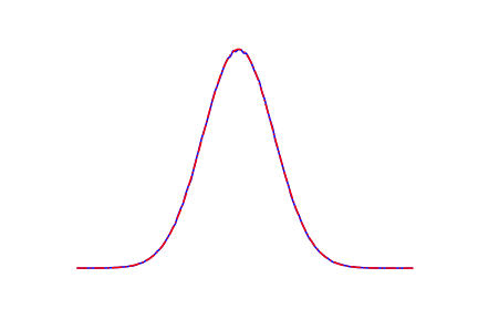
In closing, some python code:

import numpy as np
import matplotlib.pyplot as plt

dt = .01
N  = 100
l  = .05
X0 = .75

M = 1000000
res = np.zeros(M) + X0
for _ in range(N):
    res += -l*res*dt + np.sqrt(2*dt) * np.random.randn(M)

yy, xx = np.histogram(res, 128, normed=True)
plt.plot(.5*(xx[1:]+xx[:-1]), yy, 'b')
mu    = X0 * (1-l*dt)**N
sigma = np.sqrt(2*dt*(((1-l*dt)**(2*N)-1) / ((1-l*dt)**2 - 1)))
plt.plot(xx, 1./np.sqrt(2*np.pi*sigma**2)*np.exp(-(xx-mu)**2/(2*sigma**2)), 'r-.')

And the graphs go on top of each other: