Using Position Space Free particle propagator on Gaussian Wavepacket

Question

I'm teaching a class and I wanted to program a finite simulation of a quantum free particle wave packet using the free particle propagator in real space (I've used other methods in the past and wanted to do this mainly for fun). So, my strategy was to

1. Define an initial Gaussian wave packet with positive momentum $\psi_0(x, t=0)$ on a real space grid (x) that was very large.
2. Write a program that looped over each point x' in x and calculated $\psi(x',t) = \sqrt{m/2\pi it\hbar } \int{e^{i m (x-x')^2/2\hbar t} \psi_0 (x',0)dx'} $ as a simple Riemann sum
3. Plot $\psi^*\psi $ vs x to see visualize the wave packet move to the right at different times t.

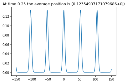
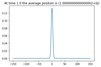
My implementation works great for large t, I see a wave packet moving to the right with speed $p_0/m$ . But for small t, clearly linked to the spacing of my grid (dx) I get recurrences I've put graphs of $\psi^*\psi$ at small time and t=1 for a particle with unit momentum and initial postional spread of $\sigma= 3$

Any thoughts on why that might be happening? I've attached my code below For example, at t=0.25

import numpy as np
import matplotlib.pyplot as plt

def gaussian(x0, sigma,p0,x):
    return np.sqrt(1/(sigma*np.sqrt(2*np.pi))*np.exp(-.5*((x-x0)/sigma)**2))*np.exp(1j * p0*x)

def free_particle_propagator(psi0,mass,x,t):
    if t < 1E-10:
        return psi0

    dx=x[1]-x[0]
    psi_t=np.zeros(psi0.shape,dtype=complex)
    for i in range(len(x)):
        psi_t[i]=np.sum(np.sqrt(mass/(2*np.pi*1j*t))*np.exp((1j*mass*(x[i]-x)**2)/(2*t))*psi0)*dx

    return psi_t
x=np.linspace(-150, 150, 10000)
dx=x[1]-x[0]

psi0=gaussian(0,3,1,x)
for time in np.linspace(0,2,25):
    psi_t=free_particle_propagator(psi0,1,x,time)
    psi2=np.real(np.conj(psi_t)*psi_t)
    plt.plot(x,psi2)
    plt.title(f'At time {time} the average position is {sum(np.conj(psi_t)*psi_t*x)*dx/norm(psi_t,x)}')
    plt.pause(0.1)