About simple thermalization simulation: why the final distribution is not $E^{2}\exp[-E/T]$ but $E\exp[-E/T]$?

Question

I made a simulation that studies the thermalization of massless particles, assuming isotropic and homogeneous spatial distribution, in 3 dimensions. Namely,

1. I started with $N$ particles having random distribution in energy $E$ and isotropic directions.

2. Next, I assumed that they meet at one point (so I drop any spatial coordinates from the exercise) and randomly chose their pairs, assuming the probability of selecting each pair is pair-independent and equal to $2/N(N-1)$.

3. Then, I generated collision kinematics: I boosted to the CM frame, and generated random polar (assuming that $\cos(\theta)$ is uniformly distributed from -1 to 1, which is true in the case of a constant matrix element of the process) and azimuthal scattering angles (simply from $-\pi$ to $\pi$), and boosted back.

4. I repeat these steps (now remembering the directions) many times.

I expected the final energy distribution of the particles to follow the scaling $E^{2}\exp[-E/T]$, where $T$ is the effective temperature of the system determined from $N$ and the total energy. $E^{2}$ comes from the Liouville theorem: the density of states in a D-dimensional space is $d^{n}\mathbf{p} \propto E^{n-1}dE$. However, I got $E\exp[-E/T]$. When repeating the same exercise for the 2D case, I got $\exp[-E/T]$ instead of $E\exp[-E/T]$.

So it looks like I missed some important point, which leads to the reduction of the dimensionality by one. What may be the reason for this?

Simulation example

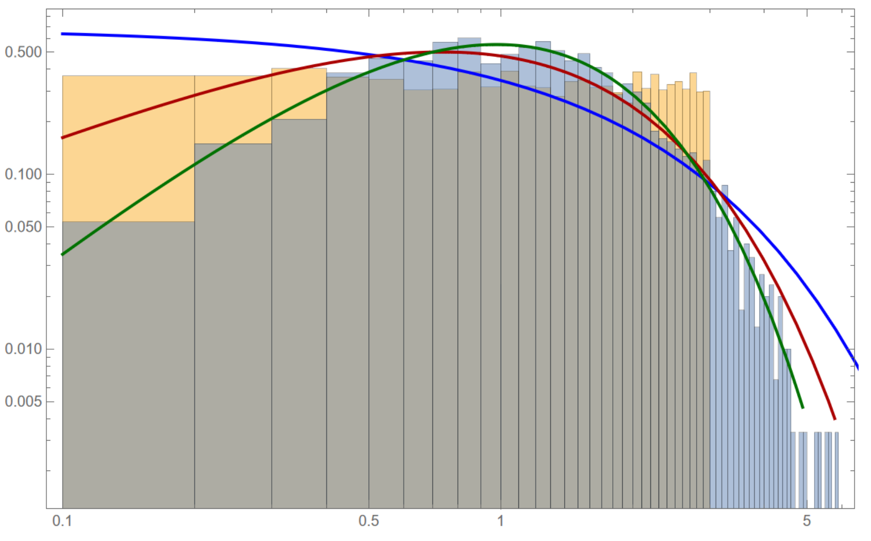
Below, there is an example of the simulation for the 3D case and identical pairing probabilities - the histogram distribution of the initial state (yellow bars), the final state (blue bars), as well as fits of the distributions $E^{n}\exp[-E/T]$ with $n = 0$ (the blue curve), $n = 1$ (the red one), $n = 2$ (the green one). For the initial distribution, I simply took $E^{2}\exp[-E/T]$:

It is clearly visible that the interactions turn the distribution from $E^{2}\exp[-E/T]$ to $E\exp[-E/\tilde{T}]$.

Also, the results do not depend on $N$ or the number of simulated steps. The system quickly falls to this "equilibrium" state, which seems like an intrinsic property of the pairing and interactions.

Answer 1

Below is my confirmation that the distribution should be proportional to $E^{n-1} e^{-E/kT}$. I originally did these calculations for massive particles, which lead to a different result than what the OP was expecting, and so I posted it as an answer. However, since my results now agree with the OP's, this no longer constitutes a possible answer, and I don't know what's going on.

---

The Boltzmann distribution in momentum space for massless particles in $n$ dimensions is $$ f(\vec{p}) \, d^n\vec{p} \propto e^{-\beta c p} \, d^n\vec{p}, $$ with $\beta = 1/kT$. To transform this into a distribution with respect to energy, we change to polar coordinates in momentum space, in which $$ d^n \vec{p} = p^{n-1} \, dp \, d\Omega_p $$ with $d \Omega_p$ representing the solid angle in velocity space. Integrating over solid angle just yields a constant that can be folded into the normalization, so the distribution with respect to speeds is $$ f(p) \, dp \propto p^{n-1} e^{-\beta cp} \, dp $$ Finally, to transform this into a distribution with respect to energy, we note that $p = E/c$ and so $dp = dE/c$; and thus $$ f(E) \, dE \propto E^{n-1} e^{-\beta E} \, dE. $$ Thus, the distribution should be $f(E) \propto E^2 e^{-E/kT}$ in 3D and $f(E) \propto E e^{-E/kT}$ in 2D.

Answer 2

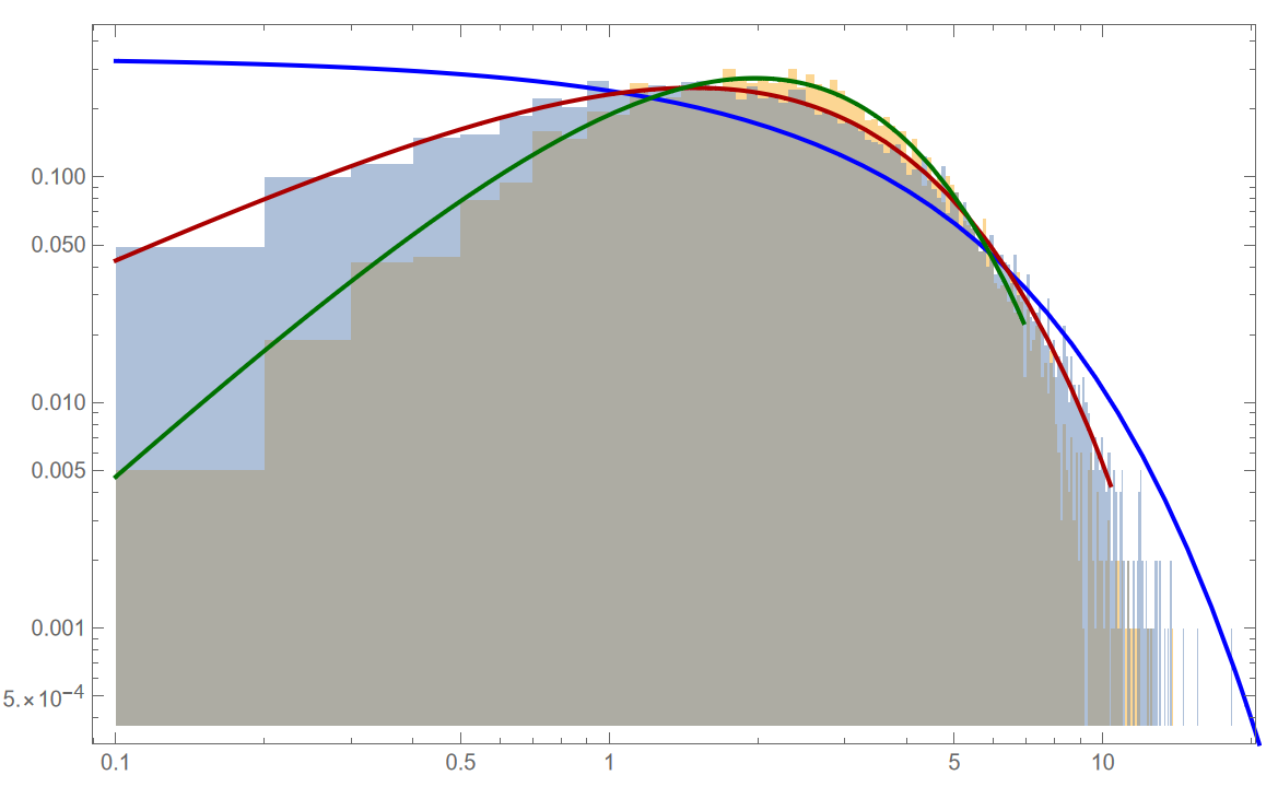
It turns out that my simulation is a simplified version of the direct simulation Monte Carlo approach (DSMC), where I restrict myself to one "particle cell". Some relevant discussions are provided in this paper; in particular, see Fig. 1 and the text around. In short, using the unit pairing weight would violate the Lorentz invariance and directly lead to the shape $\propto E\exp[-E/T]$ I got previously. So, I included the pairing weight $$ P \propto \sigma\cdot v\cdot (1-\mathbf{v}_{1}\cdot \mathbf{v}_{2}) = \frac{\sigma \cdot s}{2E_{1}E_{2}}, $$ where $$ v = \frac{p_{1}\cdot p_{2}}{E_{1}E_{2}(1-\mathbf{v}_{1}\cdot \mathbf{v}_{2})} $$ is the relative velocity, and $s$ is the invariant mass of the colliding pair.

For the particular choice $\sigma = f(s)$, I recovered the correct distribution (the plot assumes $f(s) =\text{const}$):

I would immediately break this scaling, if I include any Lorentz invariance breaking factors in the weight.