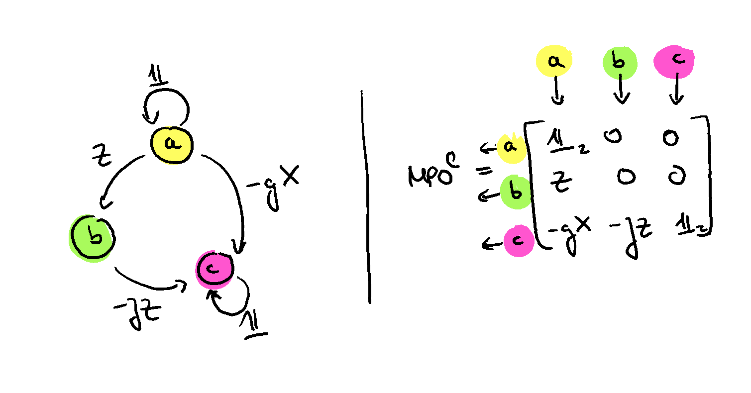
I did not check each line of the code, but it appears to me that they applied the method of using finite state automata to find the form of each local MPO. This is not possible for all Hamiltonians, but it works for many simpler models. To illustrate the idea, look at the transverse field Ising model:
$$ H = -J\sum_{\langle i,j\rangle} Z_i Z_j - g \sum_j X_j $$
From the structure of the terms one can create a finite state automaton and the corresponding matrix as

Intuitively, each application of an operator results in a change of state. Here, the successive application of $Z_j$ and $Z_i$ goes from $a$ to $b$ to $c$, while the single application of $X_j$ goes directly from the initial state $a$ to the final state $c$. Such automata can be written for many Hamiltonians, you can find some examples and explanations in this paper (interesting in this case are Fig. 3 and 4 etc.). Then, of course the MPOs at the boundary sites must be vectors, retrieved by $MPO^L = MPO^l[1,0,0]^T$ and $MPO^1 = [0,0,1] MPO^l$.
Since $MPO^l$ is a "matrix of matrices", one would write it as an array with dimensions (3,3,2,2) (depending on the convention you use). We could write in Python:
import numpy as np
g=1
J=1
X = np.array([[0,1],[1,0]])
Z = np.array([[1,0],[0,-1]])
identity = np.identity(2)
mpo_l = np.zeros((3,3,2,2))
mpo_l[0,0,:,:] = identity
mpo_l[0,1,:,:] = Z
mpo_l[0,2,:,:] = -g*X
mpo_l[1,2,:,:] = -J*Z
mpo_l[2,2,:,:] = identity
print(mpo_l)
I know that the question was asked already some time ago, but maybe this helps someone anyway.

