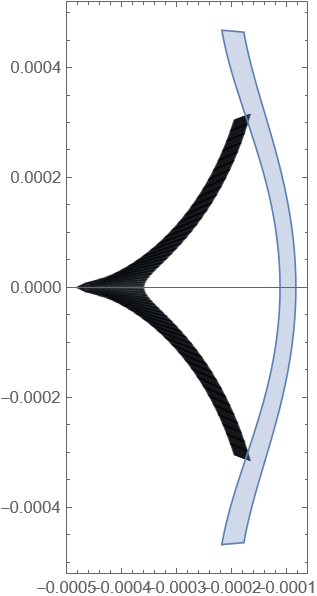
First, in the Stern-Gerlach experiment, a beam of silver atoms was used, and not a beam of electrons. Secondly, the interpretation of data at that time (1922) based on the classical equations of motion. It is assumed that the silver atom has a magnetic moment on which the force acts
$$\vec {F}=\nabla (\vec {\mu}.\vec {B})……(1)$$
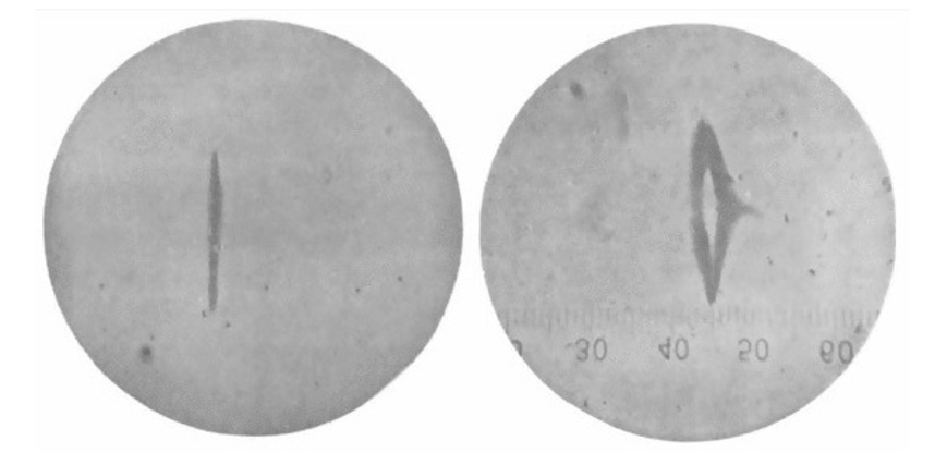
The role of quantum mechanics is reduced to the statement that the magnetic moment in equation (1) is quantized in proportion to the angular momentum or spin. In this form, the theory of the scattering of atoms in a non-uniform magnetic field was used to solve practical problems related to the determination of the magnetic moment of atoms using the Stern-Gerlach method down to the present time. As it is known, Stern and Gerlach obtained the following figure of silver atoms (on the left without a magnetic field, on the right in a magnetic field)
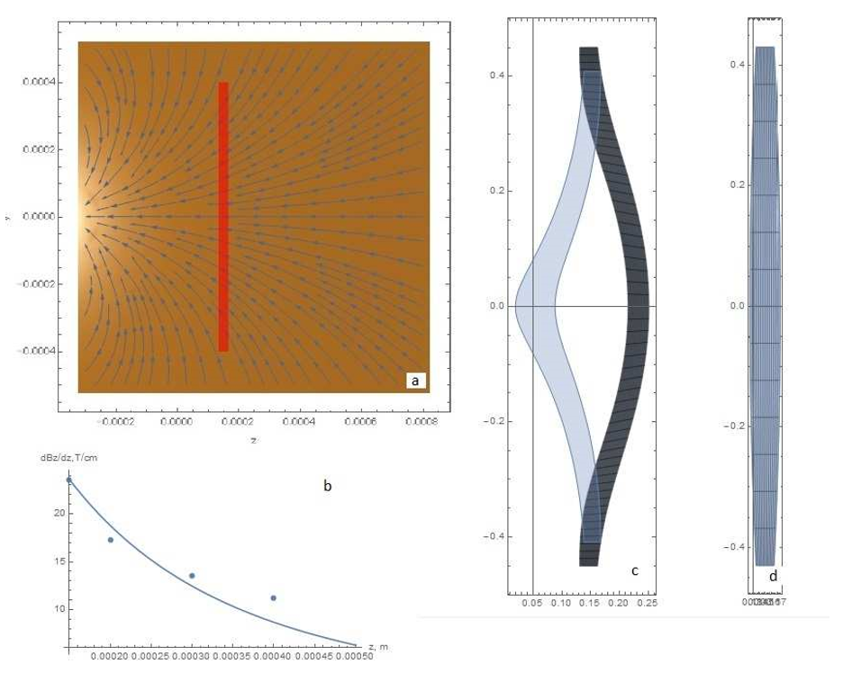
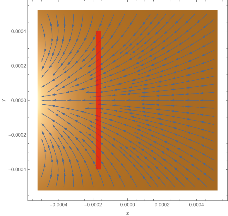
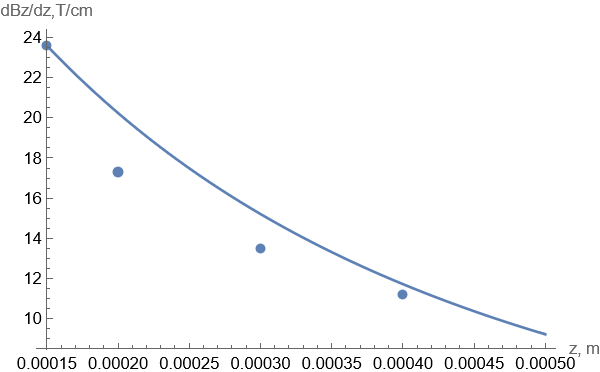
 The question is, can we get the right figure using equation (1) with $\mu =\pm \mu_B$? I simulated the scattering of silver atoms in a magnetic field with a gradient as in the Stern-Gerlach experiment. All parameters of the gap and velocity of atoms were as in experiment. The result is shown in Fig. 2, where a) magnetic field lines and gap projection (red rectangle); b)magnetic field gradient (solid line) and experimental data (points) from Stern and Gerlach; c) atomic scattering pattern in a magnetic field; d) the same without a magnetic field. Comparing the scattering figures in Figs. 1 and 2, we find that Bohr’s hypothesis about quantizing the magnetic moment with projection $\pm\mu _B$ to the direction of the magnetic field is confirmed.

A similar result can be obtained without this hypothesis, simply using the Schrödinger–Pauli equation:
$$i\hbar \frac {\partial \psi}{\partial t}=-\frac {\hbar ^2}{2m}\nabla^2\psi+\mu _B(\vec {B}.\vec {\sigma })\psi $$
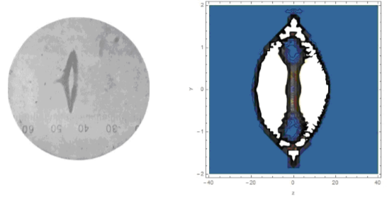
$\vec {\sigma }=(\sigma _1,\sigma _2, \sigma _3)$ there is a Pauli matrix. Figure 3 shows the scatter pattern in the quantum model.

Update 1. Data shown above have been taken from several papers and books including
W . Gerlach, O . Stern . Der experimentelle Nachweis des magnetischen Moments des Silberatoms // Zeitschrift fur Physik, 1922, Volume 8, Issue 1, pp 110 - 111.
W. Gerlach,O. Stern. Der experimentelle Nachweis der Richtungsquantelung im Magnetfeld, Zeitschrift fur Physik 9 (1922) 349-352.
The code for Mathematica shown below can be used to plot Figures as follows
Clear[p, \[Theta], \[Phi], q]
ge = .5; g = 0; L0 = .035; Wy =
 0.0008/L0; Wz = .00003/L0; nz0 = 6; eps1 = 0; eps =
 Pi/10; mB = -9.274078*10^(-24);
mAg = 107.868*1.6605655*10^(-27); kB = 1.380662*10^(-23); Tov =
 1300 + 273.15;
v0 = Sqrt[
   3.5*kB*Tov/
     mAg];(* data taken from W.Gerlach,O.Stern.Der experimentelle Nachweis des magnetischen Moments des Silberatoms//Zeitschrift fur
Physik,1922,Volume 8,Issue 1,pp 110-111*)

t1 = 1; t0 = L0/v0;

h = 1.0545887*10^(-34);
\[Omega] = mB/h;

y0 = Wz;
z0 = Wy;

f[t_] := (1 - Sign[t - t1])/2;
(*Magnetic field data taken from W.Gerlach,O.Stern. Der experimentelle Nachweis der Richtungsquantelung im Magnetfeld, Zeitschrift fur Physik 9 (1922) 349-352 *)
Bsh = {{.00015, 23.6}, {.00020, 17.3}, {.0003, 13.5}, {.0004, 11.2}};
By[y_, z_, y0_,
   z0_] := -(z + z0) (1/((y - y0)^2 + (z + z0)^2) -
     1/((y + y0)^2 + (z + z0)^2));
Bz[y_, z_, y0_,
   z0_] := (y - y0)/((y - y0)^2 + (z + z0)^2) - (y +
      y0)/((y + y0)^2 + (z + z0)^2);
Byy[y_, z_, y0_,
   z0_] := -(z + z0) (-((2 (y - y0))/((y - y0)^2 + (z + z0)^2)^2) + (
     2 (y + y0))/((y + y0)^2 + (z + z0)^2)^2);
Byz[y_, z_, y0_, z0_] := -1/((y - y0)^2 + (z + z0)^2) +
   1/((y + y0)^2 + (z + z0)^2) - (z +
      z0) (-((2 (z + z0))/((y - y0)^2 + (z + z0)^2)^2) + (
      2 (z + z0))/((y + y0)^2 + (z + z0)^2)^2);
Bzy[y_, z_, y0_,
   z0_] := -((2 (y - y0)^2)/((y - y0)^2 + (z + z0)^2)^2) +
   1/((y - y0)^2 + (z + z0)^2) + (
   2 (y + y0)^2)/((y + y0)^2 + (z + z0)^2)^2 -
   1/((y + y0)^2 + (z + z0)^2);
Bzz[y_, z_, y0_,
   z0_] := -((2 (y - y0) (z + z0))/((y - y0)^2 + (z + z0)^2)^2) + (
   2 (y + y0) (z + z0))/((y + y0)^2 + (z + z0)^2)^2;
Visualization of magnetic field and gradient
Show[{StreamDensityPlot[{Bz[y, z, y0*L0, z0*L0],
    By[y, z, y0*L0, z0*L0]}, {z, -.0005, .0005}, {y, -0.0005, .0005},
   FrameLabel -> {"z", "y"}],
  Graphics[{Opacity[.6], Red,
    Rectangle[{-z0*L0 + 21*Wz*L0 - Wz*L0/2, -Wy*L0/2}, {-z0*L0 +
       21*Wz*L0 + Wz*L0/2, Wy*L0/2}]}]}]

Show[{Plot[
   23.6*Bzz[0, z, y0*L0, z0*L0]/
     Bzz[0, .00015, y0*L0, z0*L0], {z, .00015, .0005},
   AxesLabel -> {"z, m", "dBz/dz,T/cm"}], ListPlot[Bsh]}]

Visualization of silver deposition
k = ge*mB*L0/(mAg*v0^2); k1 = k*23.6*100/Bzz[0, .00015/L0, y0, z0];
eq = {Mx'[t] ==
    f[t]*g*(Bz[y[t], z[t], y0, z0] My[t] -
       By[y[t], z[t], y0, z0] Mz[t]),
   My'[t] == f[t]*g*(-Bz[y[t], z[t], y0, z0] Mx[t]),
   Mz'[t] == f[t]*g*(By[y[t], z[t], y0, z0] Mx[t]),
   Mx[0] == Cos[\[Theta]], My[0] == Sin[\[Theta]]*Cos[\[Phi]],
   Mz[0] == Sin[\[Theta]]*Sin[\[Phi]], x''[t] == 0,
   y''[t] == (1 + .0*(y[t]/y0)^2)*f[t]*
     k1*(My[t]*Byy[y[t], z[t], y0, z0] +
       Mz[t]*Byz[y[t], z[t], y0, z0]),
   z''[t] ==
    f[t]*k1*(My[t]*Bzy[y[t], z[t], y0, z0] +
       Mz[t]*Bzz[y[t], z[t], y0, z0]), x'[0] == 1, x[0] == 0,
   y'[0] == 0, y[0] == p, z'[0] == 0, z[0] == -z0 + 21*Wz + q};
pfuny = ParametricNDSolveValue[eq,
  y[1], {t, 0, 1}, {p, \[Theta], \[Phi], q}]
pfunz = ParametricNDSolveValue[eq,
  z[1], {t, 0, 1}, {p, \[Theta], \[Phi], q}]
Show[{ParametricPlot[{Sum[
      pfunz[p, Pi/2 + eps1*j, Pi/2 + eps*j, q]*L0, {j, -nz0,
       nz0}]/(2*nz0 + 1),
    Sum[pfuny[p, Pi/2 + eps1*j, Pi/2 + eps*j, q]*L0, {j, -nz0,
       nz0}]/(2*nz0 + 1)}, { q, -Wz/2, Wz/2}, {p, -Wy/2, Wy/2},
   PlotRange -> All, Mesh -> All],
  ParametricPlot[{Sum[
      pfunz[p, Pi/2 + eps1*j, -Pi/2 + eps*j, q]*L0, {j, -nz0,
       nz0}]/(2*nz0 + 1),
    Sum[pfuny[p, Pi/2 + eps1*j, -Pi/2 + eps*j, q]*L0, {j, -nz0,
       nz0}]/(2*nz0 + 1)}, { q, -Wz/2, Wz/2}, {p, -Wy/2, Wy/2},
   PlotRange -> All, Mesh -> None]}]
