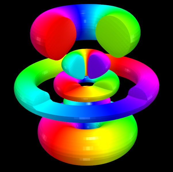
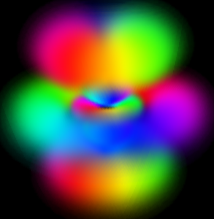
An atomic orbital is a complex function of 3D space, $\psi(x, y, z) = \psi(r, \theta, \phi)$. It is challenging to visualize 3D functions. One way to do so is to calculate the probability density $P(x, y, z) = |\psi(x, y, z)|^2$ and plot isosurface contours of $P(x, y, z)$, that is surfaces in 3D space on which $P(x, y, z) = c$ for some constant number $c$. Note that for every value of $c$ the corresponding isosurface contour "contains" a total probability $$ \text{Prob}(P(x, y, z) <= c) = \int_{|\psi(x, y, z)|^2<=c} |\psi(x, y, z)|^2 dV = p_c $$ (Note that the integration bound here is very strange. we cannot analytically calculate $p_c$ from $c$ or vise-versa, but the calculation can be done numerically without too much trouble.)
The OP seems to suggest that, when atomic orbitals are visualized, we typically choose $c$ so that $p_c=0.9$. The OP is correct that when visualizing atomic orbitals using isosurface contours we do have to choose some value for $c$ (and correspondingly a value for $p_c$). But the OP is incorrect that there is any standardized value chosen for $p_c$ across all references. See e.g. This orbital n=4, l=1, m=1 orbital on Wikipedia shown with $p_c=0.45$ (or orbital in my profile pic which shows $(n, l, m)=(4, 3, -1)$ with $p_c=0.6$). I also would suggest that $p_c=0.9$ is an uncommon value to select for $p_c$. As we'll see below, $p_c=0.9$ contains "too much" probability so that the orbitals look very "fat" and it's hard to see the geometric features of the orbital as clearly. I've found $p_c=0.6$ to be a good value for visualizing lots of different orbitals.
The OP asks:
why did we choose the points as they are, and not in a different way with a different shape made up of a different set of points that also encompasses a 90% probability of an electron being there?
The answer is that, once a probability threshold $p_c=0.9$ is selected, the wavefunction magnitude threshold $c$ such that $p_c=0.9$ is uniquely selected. The isosurface contour is then, again, uniquely selected by $|\psi(x, y, z)|^2 = c$. Most succinctly: When we see isosurface contour visualizations of atomic orbitals, those surfaces are selected so that $|\psi(x, y, z)|^2$ is constant on the surface, this is the definition of an isosurface contour.
Note that in addition to visualizing the probability $P(x, y, z)$ we can also visualize the phase of the wavefunction $\text{arg}(\psi(x, y, z))$ by coloring the portion of the isosurface contour so that the color hue maps to the wavefunction phase. i.e. phase of 0 shows up as red, phase of $\pi/2$ shows up as green, phase of $\pi$ shows up as blue, and phase of $3\pi/2$ shows up as purple. For the complex orbitals which are eigenvectors of the $L_z$ operator, this results in beautiful rainbow colored rings. for real orbitals (orbitals which are the real and imaginary parts of the complex orbitals that we often see in intro chemistry or quantum physics textbooks) this corresponds to red and blue lobes depending on whether the wavefunction is locally positive or negative.
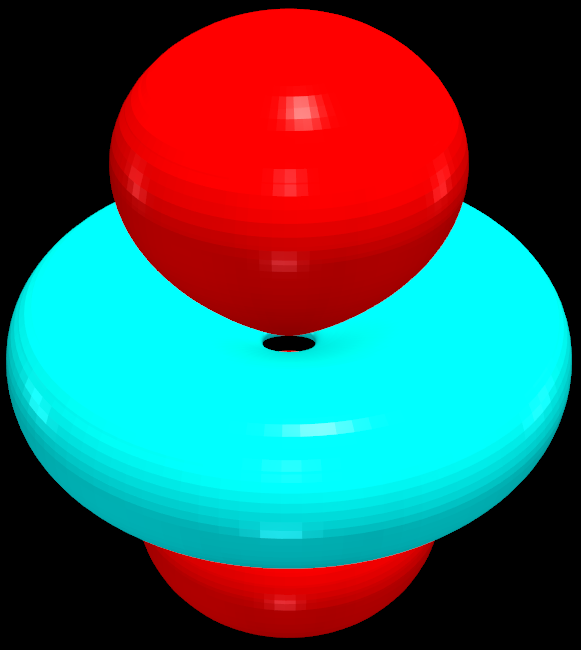
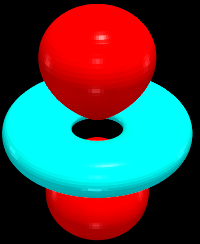
Here are some isosurface contour visualizations of the $(n, l, m) = (3, 2, 0)$ orbital.
$p_c=0.9$:
$p_c=0.6$:
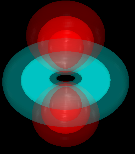
We can make the orbitals transparent with an opacity proportional to $c$ (so that more probable isosurface contours are more opaque). Below we use this technique with $p_c=0.2, 0.5, 0.8$:
Note, importantly, that we see 3 red isosurfaces, one for each probability threshold, but only 2 blue isosurfaces. This is because, at the $p_c=0.2$ level, the blue lobe is too un-probable! Thus, care must be taken to not choose a value of $p_c$ that is too low otherwise you run the risk of missing certain lower probability lobes. However, other than this constraint, we can see that the qualitative features of the orbital do not depend on the exact value chosen for $p_c$. This is why there is some "artistic freedom" we can take in selecting $p_c$ for visualizations.
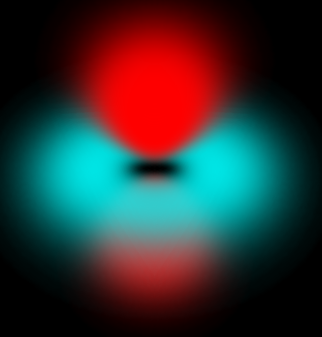
We can side-step the whole issue of selecting a value of $p_c$ by instead visualizing $\psi(x, y, z)$ as a volume cloud. In this strategy we partition space up into small voxels and set the opacity of the voxel to $\Gamma(|\psi(x, y, z)|^2dV)$ where $dV$ is the volume of the voxel and $\Gamma$ is some monotonic but possibly non-linear function that can be used to weight high or low probability regions disproportionately (again, selected based upon some artistic freedom).
Here is $(n, l, m)=(3, 2, 0)$ shown with a max opacity of 1 and a linear opacity function.
Just for fun, since I can't resist sharing these beautiful images, here are some views of the $(n, l, m) = (5, 3, 1)$ orbital. First an isosurface contour with $p_c=0.6$ with the $+x, +y, +z$ cube cutout for clarity
and a cloud volume visualization (max opacity of 1 and linear opacity function)
These images were generated using atomview, a python package I wrote which is a work in progress for me. It is based on pyvista which is a python wrapper around VTK which is itself a 3D graphics visualization framework. See Thaller, Visual Quantum Mechanics and Thaller, Advanced Visual Quantum Mechanics for more details about visualizing 3D wavefunctions, atomic wavefunction, and visualization of other quantum phenomena.

