0
$\begingroup$

I have two time series from an accelerometer attached to two different factory machines with the hope of picking up subtle differences between the machines and being able to tell when a machine should undergo maintenance before it actually breaks down. My initial idea was to do a Fourier transform of the time series and look at the eigen frequencies of the machines and hopefully be able to pick up something based on that. However, it has been more than a decade since I finished my master in physics and I haven't used the fourier transform in a long time, so I'm quite rusty in this.

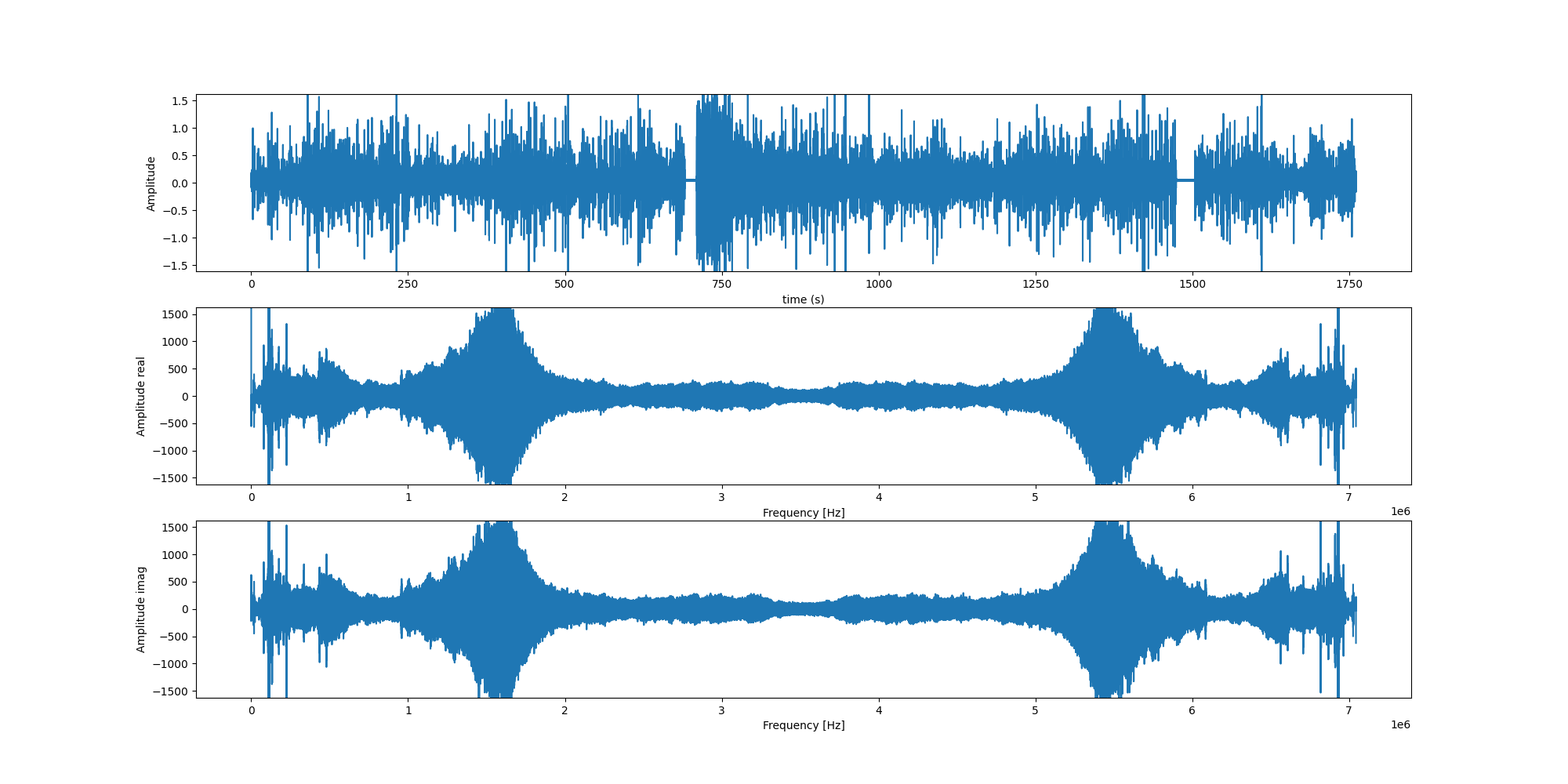
enter image description here

The top row is the time series itself, while the bottom 2 rows are the real and imaginary component of the FFT.

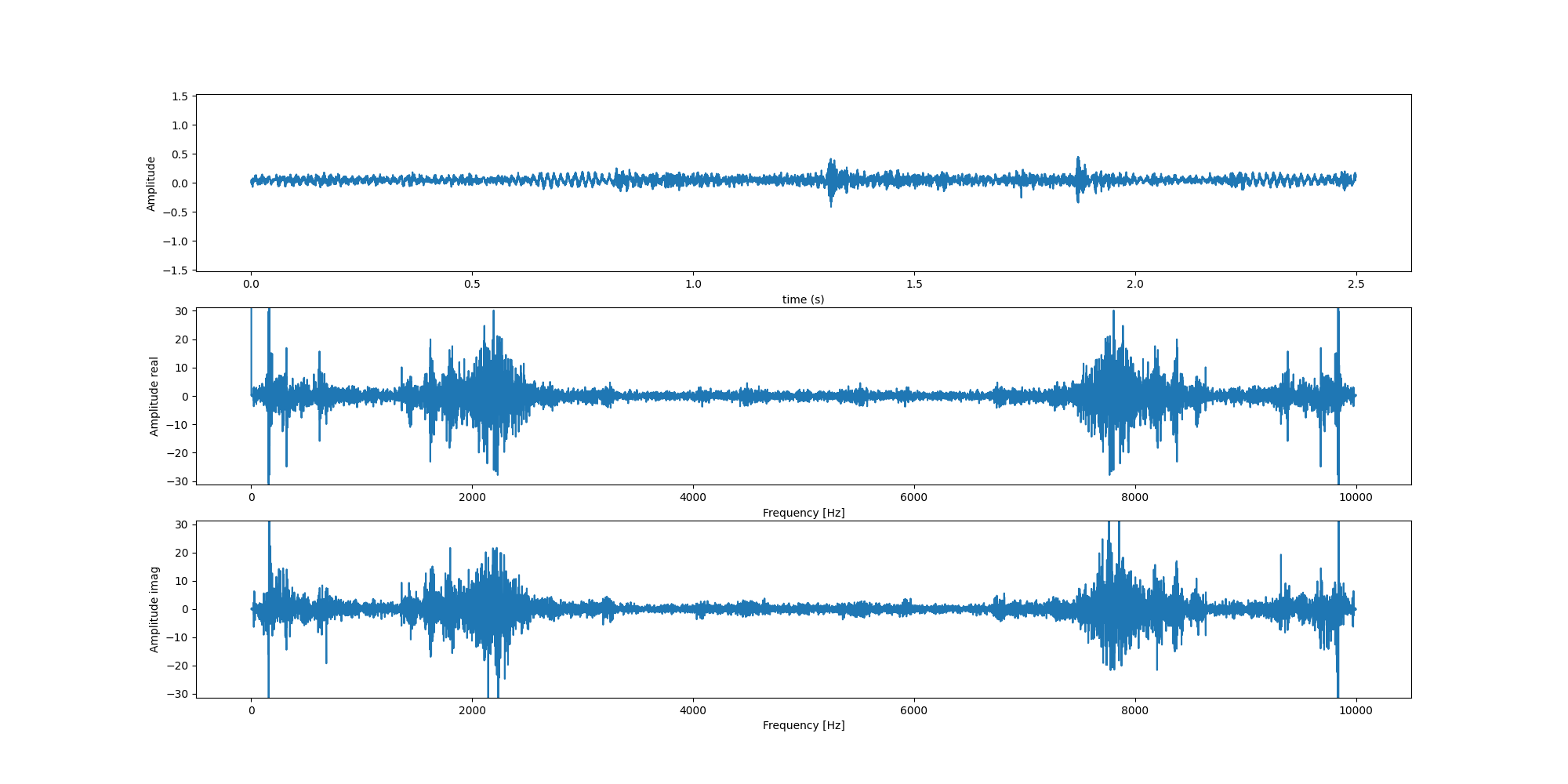
enter image description here

Same as the above, but this time on a small subsection of the data limited to only 10000 samples.

My data is sampled at 1/4000 s and my initial attempt was just to take the fourier transform directly of this time series, as well as some subsets of the time series. However, the Fourier transforms I get from this looks weird to me. Why is the fourier transform essentially symmetric about the halfpoint of the x-axis? This seems un-physical to me and likely means I'm doing something stupid.

Right now I'm just using numpy's FFT algorithm directly on the data, and I don't see anything in the documentation to suggest I should be doing something else.

What am I missing?

$\endgroup$

1 Answer 1

1
$\begingroup$

This isn't a physics question, but, I like numpy.fft, and I use it a lot at work.

So FFTs are complex, and transform a complex signal to positive and negative frequencies.

Your machine is real, and your time series is real, with that, the coefficients have a symmetry:

$$ c_{+f} = c_{-f} $$

so that the motion at $|f|$ comes from:

$$c_{+f}e^{2\pi ift} + c_{-f}e^{-2\pi ift}$$

$$ (c_{+f} + c_{+f})\cos{2\pi ft} + i (c_{+f} - c_{+f})\sin{2\pi ft} = 2c_{+f}\cos{2\pi ft}$$

is real, as it must be.

For complex FFTs, the standard is to have the frequency axis go as [0, 1, 2, 3, ..., -3, -2, -1] and can be accesses with np.fft.fftfreq function.

But, you can by pass all that by using real FFTs:

So:

  1. use numpy.fft.rfft (real FFT's)

  2. numpy.fft.rfttfreq to get the frequency axis for (1)

Now that fft is still complex, because the there is phase information required to do the inverse FFT. You probably don't care about that, so you want the absolute value (maybe squared), at which point you are computing power-spectral densities.

Here you should see power at various frequencies of interest, e.g, there should be a peak at 60 Hz and maybe harmonics thereof associated with AC power affecting everything.

If there is temperature dependence, you may see power at 24 hours, or seasonally-- I look at 20 year time series from satellites, and you got power at these very low frequencies, including a lunar correlation, and at the orbit frequency (1/LEO).

See also the "Periodogram"--which is slightly different than a PSD, but really, the information is the same.

If you have long term drift with 1/f noise, then you can use Allan variance to get a handle on that.

$\endgroup$
1
  • $\begingroup$ This was such a great answer, thank you very much for the detailed explanation! $\endgroup$
    – Tue
    Commented Sep 17 at 7:53

Your Answer

By clicking “Post Your Answer”, you agree to our terms of service and acknowledge you have read our privacy policy.

Not the answer you're looking for? Browse other questions tagged or ask your own question.