Mean field theory Vs Gaussian Approximation?

Question

I am getting confused about the distinction between Mean-field theory (MFT) and the Gaussian approximation (GA). I have being told on a number of occasions (in the context of the Ising model) that the Gaussian approximation is at the same level as MFT.

I think this refers to the mean-field theory associated with $$ H = -J \sum_{\langle i,j \rangle} \big( (\sigma_i-M) + M \big) \big( (\sigma_j - M) + M \big) ~, \tag{1} $$ where $M$ is the mean-field, and $(\sigma - M)$ represent the fluctuations. but then I have also read that the GA is the lowest order correction to the MFA — i.e., found with the saddle-point method; consult Kopietz et al. “Introduction to the functional renormalization group”. Springer (2013) [wcat].

How do these two agree? Is the MFT associated with (1) really on the same level as the GA which is at a higher level than the MFT associated with the saddle-point approximation? Or am I missing something?

Edit

The answers as they currently stand (23/03/2018) simply give (exactly or almost exactly) what is in the reference that I gave in this question - and as such this is clearly something I have seen before. This reference does explain (as I have said in my question) that the GA is a correction to the saddle point MFA. But does not mention anything about the MFA in (1) and how it relates to the GA - which is basically the crux of my question.

Answer 1

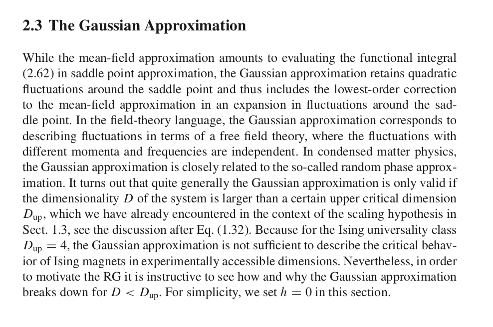
The mean-field approximation amounts to evaluating the functional integral for the partition function in saddle point approximation, while the Gaussian approximation retains quadratic fluctuations around the saddle point and thus includes the lowest-order correction to the mean-field approximation in an expansion in fluctuations around the saddle point.

The Gaussian approximation is closely related to the random phase approximation, especially in the context of quantum many-body systems, while the mean-field approximation in that case might be seen as the self-consistent Hartree–Fock approximation.

The reason for the confusion may be that the Gaussian approximation is only valid if the dimensionality of the system is larger than a certain upper critical dimension. Because for the Ising universality class this dimension is 4, the Gaussian approximation is not sufficient to describe the critical behavior of Ising magnets in experimentally accessible dimensions, which is why perhaps you might have been told it's on the same level as the mean-field approximation?

Answer 2

Here is a book chapter to solve your problem: Kopietz et al. “Mean-Field Theory and the Gaussian Approximation”. Lect. Notes Phys. 798, 23–52 (2010) [PDF].

Answer 3

A quantum field theory is modeled by a probability distribution (measure) over the space of all field configurations, specified implicitly by an action functional. We seek to describe systems by characterizing their distributions using moments (correlation functions).

A simple characterization for the multi-variate distribution (each point corresponds to one random variable) is to specify it's mean at every point in space. The mean field approximation does exactly that -- it neglects all "fluctuations" in field values at each point and considers a classical "field profile". Commonly, this field profile is also assumed to be uniform in space, so that one may conveniently solve for self-consistent answers for the background field value. Also, note that such a solution (lowest action configuration i.e. max-likelihood, as is usually computed in physics) is actually the "mode" of the distribution -- but the mode and the mean are interchangeable if the distribution is peaked and large fluctuations have negligible measure. (Note: If the system is not in that regime, then these approximations/truncations are useless anyways, so splitting hairs regarding the terminology here is quite pointless)

Quantum mechanically, the true solution is the superposition of a bunch of configurations which are modeled as "fluctuations" around the "mean" field. Neglecting any interactions between these fluctuations at different points (suppressed by a coupling constant) the leading order dynamics is captured by a quadratic Lagrangian — just the kinetic/gradient terms for the fluctuations. As this action leads to a Gaussian measure on the fluctuating degrees of freedom, it is also referred to as the Gaussian approximation. This is equivalent to treating each fluctuation degree of freedom as an independent harmonic oscillator (essentially "free" field theory).

Whether each of these approximations is useful depends on details like the size of the coupling constant, dimensionality of the system, etc. The essence of all those conditions comes down the whether the effect of fluctuations is sufficiently controlled/negligible. A common theme in statistical physics is the applicability of these approximations in one parameter regime, and the dominance of fluctuations in another regime, with a phase transition as the appropriate description changes from one renormalization group basin of attraction to another.

Answer 4

I couldn't do the comment, so I will just answer here about your edit.

The reference you mentioned ("Introduction to the Functional Renormalization Group", link) actually do the full analysis for the MFA and GA of the Ising model you wrote down. I think the part you might have missed is the section 2.2.2, where the authors do the $\phi^4$ truncation to the Ginzburg-Landau free energy. From there, you can follow section 2.1.2 to do the MF analysis, which corresponds to solving the Euler-Lagrange equation. After that, they do the GA correction of free energy following section 2.3.1 by expanding the field configuration around the MF solution to the quadratic order and do the Gaussian integration.

Following the calculation, it should be clear that the last Gaussian integration contributes an extra term to the free energy after the mean field part, and thus it is the leading order correction (though not controlled error generally).

As for your original question: "on a number of occasions (in the context of the Ising model) that the Gaussian approximation is at the same level as MFT.", it is shown in the book that for D>4 there is actually no correction to the critical exponents at all.

Answer 5

Whether or not the two approximations are equivalent depends on what you're trying to calculate. Formally, the Gaussian approximation always produces one term beyond the mean-field approximation. However, in some applications that additional term doesn't actually depend (nontrivially) on the couplings that you care about, so it just adds a constant to the action and does not affect any physical observables. For example, Kopietz section 2.3.2 says

Gaussian fluctuations do not modify the mean-field predictions for the exponents β, γ , and δ, which are related to the homogeneous order-parameter fluctuations. Within the Gaussian approximation, we therefore still obtain β = 1/2, γ = 1, and δ = 3. On the other hand, the Gaussian approximation for the specific heat exponent α is different from the mean-field prediction α = 0, because the fluctuations with finite wave vectors give a nontrivial contribution Δf to the free energy per lattice site.

In some calculations (e.g. the replica trick for disordered systems), we have an action of the form $Z = \int D\varphi\ e^{-\beta N f[\varphi]}$, where the free energy density $f$ does not depend on the system size $N$. In this case the mean-field approximation $Z \propto e^{-\beta N f(\bar{\varphi})}$ actually becomes exact in the large-$N$ thermodynamic limit, and the Gaussian corrections manifest themselves as finite-size corrections, which we rarely care about.

Answer 6

In the thermodynamic limit the mean field result of the ising model becomes exact. Since the Gaussian approximation includes corrections to the mean field you can use this technique to show that these corrections vanish in the thermodynamic limit. In this scence the mean field an gaussian approximation are identical in the thermodynamic limit since they are both exact.