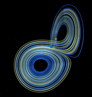
The first dynamics is not chaotic
The rotation around an intermediate axis was analysed by Ashbaugh et al., J. Dyn. Diff. Eq. 3 (1), pp. 67–85. They describe the phenomenon using the following differential equations:
$$ \begin{align}
\dot{θ} &= - M \left( \frac{1}{I_1} - \frac{1}{I_3} \right) \sin(θ) \sin(ψ) \cos(ψ)\\
\dot{ϕ} &= \frac{M}{I_3} \sin^2(ψ) + \frac{M}{I_1} \cos^2(ψ)\\
\dot{ψ} &= \left( \frac{M}{I_2} - \frac{M \sin^2 (ψ)}{I_3} - \frac{M \cos^2(ψ)}{I_1} \right)\cos(θ)
\end{align}$$
Obviously, $ϕ$ does not appear on the right-hand side of the equation. In particular, $ϕ$ is not relevant to describe the dynamics of $θ$ and $ψ$, which can be described by a two-dimensional system (which then drives $ϕ$). As two-dimensional systems cannot exhibit chaos, this also means that the system in question cannot be chaotic. Instead, $θ$ and $ψ$ exhibit a periodic dynamics. And just in case, somebody is skeptical: Simulations confirm this¹. This can also be seen in the video: The flipping is pretty regular.
Why the trajectory is area-filling
As $\dot{ϕ}$ is completely governed by a periodic process, one might naïvely expect that the entire system is also periodic. However, the frequency of the dynamics of $θ$ and $ψ$ does not seem to be commensurable by the frequency of time points at which $ϕ$ is a multiple of $2π$ (in a simulation¹). Therefore $ϕ \bmod 2π$ exhibits a quasi-periodic behaviour, which is indeed capable of filling a surface.
¹ Here is the source code of a Python simulation, if anybody wants to play with this system:
from jitcode import jitcode_lyap, provide_basic_symbols
from scipy.stats import sem
import numpy as np
from sympy import sin, cos, atan, sqrt

I_1, I_2, I_3 = 0.00121, 0.01638, 0.01748
E = 0.32333

θ_0 = np.random.uniform(0,0.025)
ψ_0 = np.random.uniform(0,np.pi)
φ_0 = atan( -sin(ψ_0) / cos(ψ_0) / cos(θ_0) )
M = sqrt( 2 * E / (cos(ψ_0)**2 * sin(θ_0)**2 / I_1 + cos(θ_0)**2 / I_2 + sin(ψ_0)**2 * sin(θ_0)**2 / I_3))

t, y = provide_basic_symbols()
θ,φ,ψ = y(0),y(1),y(2)

f = [
    -M * (1/I_1-1/I_3) * sin(θ) * sin(ψ) * cos(ψ),
    M / I_3 * sin(ψ)**2 + M / I_1 * cos(ψ)**2,
    ( M / I_2 - M * sin(ψ)**2 / I_3 - M * cos(ψ)**2 / I_1 ) * cos(θ)
    ]

n = len(f)
ODE = jitcode_lyap(f, n_lyap=n)
ODE.set_integrator("dopri5")
ODE.set_initial_value([θ_0, φ_0, ψ_0], 0.0)

states = []
lyaps  = []
for time in np.arange(0.01,10000,0.01):
    state, lyap, _ = ODE.integrate(time)
    states.append(state % (2*np.pi))
    lyaps.append(lyap)

np.savetxt("timeseries.dat", states)

#converting to Numpy array for easier handling
lyaps = np.vstack(lyaps)
for i in range(n):
    lyap = np.average(lyaps[10:,i])
    stderr = sem(lyaps[10:,i]) # Note that this only an estimate
    print("%i. Lyapunov exponent: % .6f ± %.6f" % (i+1,lyap,stderr))


