Emissivity of the material certainly does play a role. Also, if the material is particularly reflective, you might get stray energy bouncing in from the surrounding (i've seen this happen with aluminum).
If your sensor absorbed all radiation, you'd use the Stephan-Boltzman law, as you've mentioned. The trick that you need is to find the fraction of the energy that is stored in band of interest. For this you'd look at Planck's law, which lets you find the energy as a function of wavelength:
$$ B(T, \lambda) = \frac{2hc^2}{\lambda^5} \left[ e^{ \frac{hc}{\lambda k_B T} } -1 \right]^{-1} $$
so the fraction of the total energy emitted in your band becomes like an effective emissivity
$$ \epsilon_{eff} (T) = \frac{\int_{\lambda_1}^{\lambda_2}B(T, \lambda)d\lambda}{\int_{0}^{\infty}B(T, \lambda)d\lambda} $$
that you use with the S.B. law so that the signal from your sensor is:
$$V(T) = C_{cal} \,\epsilon_{eff}(T) \,T^4$$
I've avoided all of the solid angle inegrations involved with these intergral (as you'd see in the derivation of $\sigma$) under the assumption that you'll need to take at least one calibration measurement (with the target at known $T$) in order to account for optics, sensor sensitivity etc. anyway. The calibration constant $C_{cal}$ takes care of all of those shenanigans.
Distance will not change the result. Although energy reaching the lens goes as $d^{-2}$ (becoming smaller as you move away), that energy is concentrated over a smaller area on the imaging plane, also going as $d^{-2}$. So the flux incident on a given pixel remains constant (registering as the same temperature).
This will hold true until the image of the object becomes smaller than one pixel. At that point the average flux at the pixel will start to drop and temperature will appear to fall.
Note: because of the peak-shape of the black body curve, it is possible for some combinations of temperature ranges and sensor bandwidths that $e_{eff}$ could be non-monotonic, introducing ambiguity by allowing $V(T)$ to have the same value at different temperatures. A quick plot of the expected curve in advance will let you know if that'll be a problem.

