3
$\begingroup$

I am trying to get a deeper understanding of Liouville's theorem and the distribution function in general. As an aid, I was thinking of the following simple, one-dimensional case: ball bearings are dropped from rest from some height at a constant rate. My understanding of the distribution function is that it gives the density of particles in phase space (here x-v space where x is the distance below drop site), and the fact that the particles are non-interacting means that the total time derivative of the distribution function is zero. As I understand it, the total time derivative of the distribution function being zero is another way of saying that if you follow any one particle then the density of particles in phase space near that particle does not change as the particle follows its trajectory.

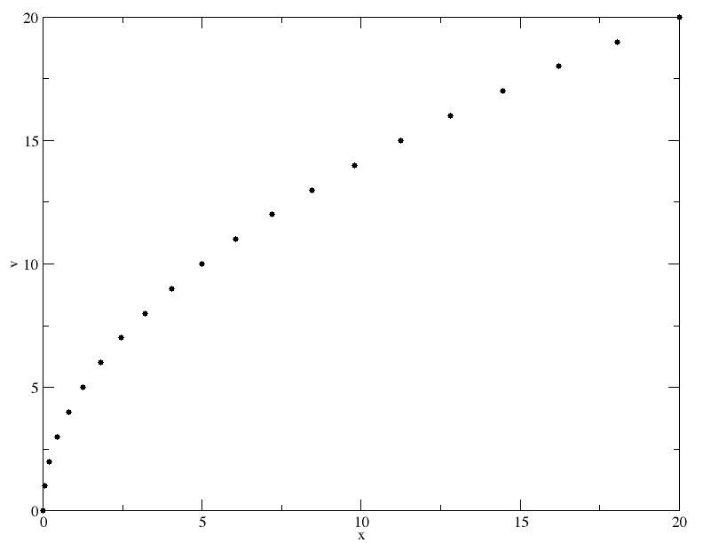
Assuming this is all correct, where I am having trouble is understanding why it appears to me that the phase space density decreases with distance from the drop site for my simple example. I have attached a phase space plot showing a single particle's position and momentum at equal time steps from release. If many particles are released at regular (small) intervals, it seems clear from this plot that the density of particles in phase space would decrease as the particles get further away from the origin, which is counter to Liouville. There must be some hole in my logic! Is anyone willing to point out where I go wrong?

Edit: after the comment was made about the plot I edited the second paragraph to attempt to clarify what is being shown

$\endgroup$
6
  • $\begingroup$ I'm a little unclear on what's going on here. What exactly is being plotted? $\endgroup$ Commented Apr 16, 2018 at 20:55
  • $\begingroup$ Sorry, I wasn't very clear. It is a plot of particle phase space (velocity vs. position). If particles are released at constant interval from the origin from rest and one takes a snap shot some time later, this shows the distribution of those particles in phase space when the snap shot is taken. Spacing between particles should be indicative of phase space density. $\endgroup$
    – Damon
    Commented Apr 16, 2018 at 21:06
  • $\begingroup$ Is this really a Hamiltonian flow? At t=0 the density is zero, as your plot shows. What are your boundary conditions at the bottom of your system? $\endgroup$
    – JohnS
    Commented Apr 16, 2018 at 22:32
  • $\begingroup$ I don't really understand the question. I'm sorry. This could be thought of as a waterfall problem in two-dimensions. In the y-direction is a constant velocity river of particles that approaches a cliff. The origin in the plot is where the particles go off the cliff (all x=0 before the cliff, so not zero density but high density). This turns it to a 4D phase space, but the y-velocity is constant and the spacing between points in vy is constant. The changes in the phase space density are only those from this plot. I don't know that this helps! $\endgroup$
    – Damon
    Commented Apr 16, 2018 at 22:43
  • $\begingroup$ Liouville's theorem states that phase space volume is preserved by the Hamiltonian flow. If I understand correctly, you are considering an initial particle distribution that has zero volume (it's just the sum of a few $\delta$-functions). The volume is still zero after time-evolving the system. $\endgroup$ Commented Apr 17, 2018 at 3:15

2 Answers 2

2
$\begingroup$

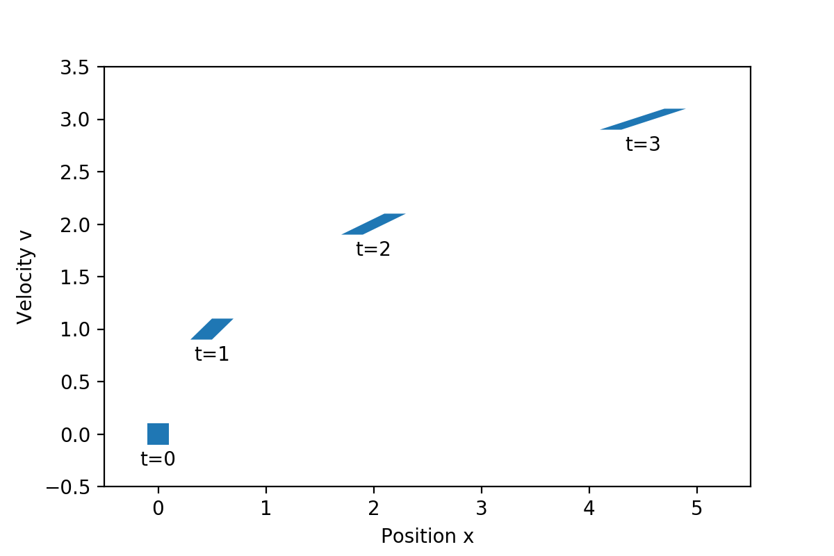
As already pointed out in the comments, there is not contradiction: your initial distribution is a single point in phase space, and so is the distribution at future times. Therefore the phase space volume is conserved.

A more revealing illustration is to see what happens to a small phase space area element (not a single point) under time evolution. For example, assume the initial distribution is a rectangle $\{(x,v):x_0-dx \leq x \leq x_0 + dx \text{ and } v_0 - dv \leq v \leq v_0 + dv \}$. As time progresses this rectangle will deform, but its area will not change (assuming $dx$ and $dv$ are sufficiently small):

enter image description here

Here is the python code to create this figure:

import numpy as np
import matplotlib.pyplot as plt
from matplotlib.patches import Polygon

a = 1.0             # acceleration
x0, v0 = (0.,0.)    # center of initial phase space element
dx, dv = (0.1,0.1)  # (half of) width of initial phase space element

p0 = np.array(((x0-dx,v0-dv),(x0-dx,v0+dv),(x0+dx,v0+dv),(x0+dx,v0-dv)))     # initial phase space element

def propagate(p0, t):
    """Propagates a phase space patch p0 for time t."""
    x0, v0 = p0.T
    x = x0 + v0*t + 0.5*a*t**2
    v = v0 + a*t
    return np.column_stack((x,v))

fig = plt.figure()
ax = fig.add_subplot(111)
for t in np.arange(4):
    p = propagate(p0,t)
    ax.add_patch(Polygon(p))
    x, y = np.mean(p,axis=0)
    plt.text(x, y-0.3, "t={}".format(t), horizontalalignment='center')
ax.set_xlabel("Position x")
ax.set_ylabel("Velocity v")
ax.set_xlim(-0.5,5.5)
ax.set_ylim(-0.5,3.5)
plt.show()
$\endgroup$
1
  • $\begingroup$ This is a beautifully concise and clear response. Thank you. Very illustrative. This really helped to clear things up for me. Thank you! $\endgroup$
    – Damon
    Commented Apr 17, 2018 at 16:59
0
$\begingroup$

The hole in your logic. @user8153 's illustrative answer is impeccable, but let me flesh out the relevant part of it --"where did I go wrong?".

Geometry.

You are considering trajectories solving $\dot{v}=g$ and $\dot{x}=v$ in funny units; let me take $g=1$ here for simplicity. You are plotting the trajectory $(x,v)$ through the origin, $(t^2/2,t)$ and releasing ball bearings at fixed intervals T. You are puzzled that phase-space points corresponding to adjacent releases $t=nT$ and $t=(n-1)T$ for $nT\gg 1$ present as drifting apart. (You may estimate the distance on the trajectory, the hypotenuse of the relevant right triangle of these two points to have length $nT^2=tT$, so to be growing linearly in time.)

But flows in phase space notoriously shear, and lots of linear dimensions, actually, increase. A phase-space density, however, is inversely proportional to an area, for which you need at least three points. So let us monitor yet another point, and hence the area of the triangle these three points define.

So, beyond points A, $((n-1)^2T^2/2,(n-1)T)$, and B, $(n^2T^2/2,nT)$, implicitly defined above, start with a point C of the trajectory above yours with a small downward push, initial velocity s, $(t^2/2+st,t+s)$.

The edges connecting A-B, and C-A, then are $((n+1/2)T^2,T)$ and $(sTn,s)$. The area of the phase-space triangle thus defined is half the 2D cross product thereof, i.e., $sT^2/2$. Dependence on $n$, so, then, $t$ has dropped out, indicating constant phase space area, and hence density.

$\endgroup$
2
  • $\begingroup$ Thank you, Cosmas. This was very helpful in thinking about this and a clever way to show the shearing algebraically. I am only allowed to give one check mark, and unfortunately the pretty picture won the day, but this was also a really nice way to present the argument. Thank you for taking the time to write it up. Very helpful! $\endgroup$
    – Damon
    Commented Apr 17, 2018 at 17:02
  • 1
    $\begingroup$ I upvoted both answers, but they don't count until I reach a 15 reputation: a lofty goal I hope to reach! $\endgroup$
    – Damon
    Commented Apr 17, 2018 at 19:45

Your Answer

By clicking “Post Your Answer”, you agree to our terms of service and acknowledge you have read our privacy policy.

Not the answer you're looking for? Browse other questions tagged or ask your own question.