Return to Answer

It looks fine to me. 2. and 3. are surely correct. 1 seems good too from your link and works well for a Wiener process where you indeed find that from your formula that MSD$\sim t$.

Concerning your example, it's pretty far from a regular Brownian motion. If we have the following Brownian motion, with $\eta$ a Gaussian random noise:

$$\dot x(t) = \eta(t)\tag 1$$

We obtain: $S_{x}(w) = S_\eta(w)/w^2$. In your case, this would imply that the noise has a spectrum:

$$S_\eta(w) = S\Theta(\Omega-|w|)w^2 \tag 2$$

And thus an auto-correlation (for $t>0$):

$$S_{\eta}(t) = S\dfrac{4t\Omega \cos(t\Omega)+2((t\Omega)^2-2)\sin(t\Omega)}{t^3} \tag 3$$

I'm sure the double integral required to obtain the MSD from (3) can be done, but I'm lazy so I just asked python to do it numerically. And here is what we obtain ($S = 1$ and $\Omega = 1$):

So your formula is indeed right! As a rule of thumb, any system driven by a noise with power law autocorrelation will display highly non diffusive behavior (usually you obtain sub or super diffusion, not "no diffusion at all"). Here the finite MSD, I think is due to the fact that your noise can easily be anticorrelated which implies that if you start to explore some region, it is highly likely that in the future you will just go back to where you were before.

It looks fine to me. 2. and 3. are surely correct. 1 seems good too from your link and works well for a Wiener process where you indeed find that from your formula that MSD$\sim t$.

Concerning your example, it's pretty far from a regular Brownian motion. If we have the following Brownian motion, with $\eta$ a Gaussian random noise:

$$\dot x(t) = \eta(t)\tag 1$$

We obtain: $S_{x}(w) = S_\eta(w)/w^2$. In your case, this would imply that the noise has a spectrum:

$$S_\eta(w) = S\Theta(\Omega-|w|)w^2 \tag 2$$

And thus an auto-correlation (for $t>0$):

$$S_{\eta}(t) = S\dfrac{4t\Omega \cos(t\Omega)+2((t\Omega)^2-2)\sin(t\Omega)}{t^3} \tag 3$$

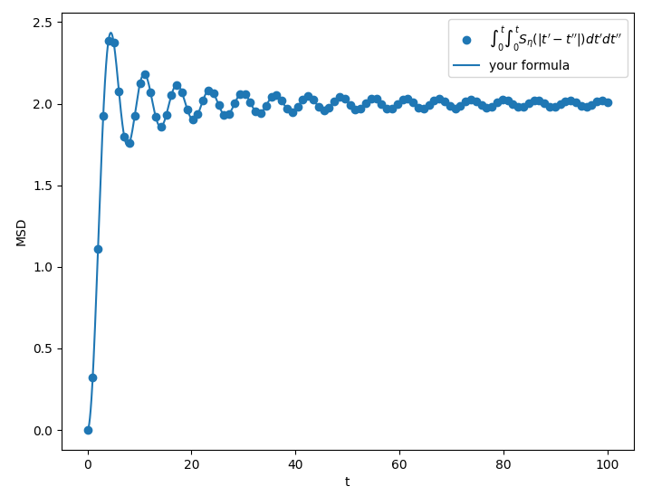
I'm sure the double integral required to obtain the MSD from (3) can be done, but I'm lazy so I just asked python to do it numerically (see edit). And here is what we obtain ($S = 1$ and $\Omega = 1$):

So your formula is indeed right! As a rule of thumb, any system driven by a noise with power law autocorrelation will display highly non diffusive behavior (usually you obtain sub or super diffusion, not "no diffusion at all"). Here the finite MSD, I think is due to the fact that your noise can easily be anticorrelated which implies that if you start to explore some region, it is highly likely that in the future you will just go back to where you were before.

Edit

Just for completeness, I'll do the integral (which in any case is already done in your linked post):

$$MSD(t) = \int_0^t\int_0^tS_\eta(|t'-t''|)dt'dt''.$$

By symmetry:

$$MSD(t) = 2\int_0^tS_\eta(u)(t-u)du=2S\Omega(1-\text{sinc}(\Omega t))$$

as expected.

It looks fine to me. 2. and 3. are surely correct. 1 seems good too from your link and works well for a Wiener process where you indeed find that from your formula that MSD$\sim t$.

Concerning your example, it's pretty far from a regular Brownian motion. If we have the following Brownian motion, with $\eta$ a Gaussian random noise:

$$\dot x(t) = \eta(t)\tag 1$$

We obtain: $S_{x}(w) = S_\eta(w)/w^2$. In your case, this would imply that the noise has a spectrum:

$$S_\eta(w) = S\Theta(\Omega-|w|)w^2 \tag 2$$

And thus an auto-correlation (for $t>0$):

$$S_{\eta}(t) = S\dfrac{4t\Omega \cos(t\Omega)+2((t\Omega)^2-2)\sin(t\Omega)}{t^3} \tag 3$$

I'm sure the double integral required to obtain the MSD from (3) can be done, but I'm lazy so I just asked python to do it numerically. And here is what we obtain ($S = 1$ and $\Omega = 1$):

So your formula is indeed right! As a rule of thumb, any system driven by a noise with power law autocorrelation will display highly non diffusive behavior (usually you obtain sub or super diffusion, not "no diffusion at all")

It looks fine to me. 2. and 3. are surely correct. 1 seems good too from your link and works well for a Wiener process where you indeed find that from your formula that MSD$\sim t$.

Concerning your example, it's pretty far from a regular Brownian motion. If we have the following Brownian motion, with $\eta$ a Gaussian random noise:

$$\dot x(t) = \eta(t)\tag 1$$

We obtain: $S_{x}(w) = S_\eta(w)/w^2$. In your case, this would imply that the noise has a spectrum:

$$S_\eta(w) = S\Theta(\Omega-|w|)w^2 \tag 2$$

And thus an auto-correlation (for $t>0$):

$$S_{\eta}(t) = S\dfrac{4t\Omega \cos(t\Omega)+2((t\Omega)^2-2)\sin(t\Omega)}{t^3} \tag 3$$

I'm sure the double integral required to obtain the MSD from (3) can be done, but I'm lazy so I just asked python to do it numerically. And here is what we obtain ($S = 1$ and $\Omega = 1$):

So your formula is indeed right! As a rule of thumb, any system driven by a noise with power law autocorrelation will display highly non diffusive behavior (usually you obtain sub or super diffusion, not "no diffusion at all"). Here the finite MSD, I think is due to the fact that your noise can easily be anticorrelated which implies that if you start to explore some region, it is highly likely that in the future you will just go back to where you were before.

It looks fine to me. 2. and 3. are surely correct. 1 seems good too from your link and works well for a Wiener process where you indeed find that from your formula that MSD$\sim t$.

Concerning your example, it's pretty far from a regular Brownian motion. If we have the following Brownian motion, with $\eta$ a Gaussian random noise:

$$\dot x(t) = \eta(t)\tag 1$$

We obtain (up to some $2\pi$ factors): $S_{x}(w) = S_\eta(w)/w^2$. In your case, this would imply that the noise has a spectrum:

$$S_\eta(w) = S\Theta(\Omega-|w|)w^2 \tag 2$$

And thus an auto-correlation (again up to some $2\pi$ factor and for $t>0$):

$$S_{\eta}(t) = S\dfrac{4t\Omega \cos(t\Omega)+2((t\Omega)^2-2)\sin(t\Omega)}{t^3} \tag 3$$

I'm sure the double integral required to obtain the MSD from (3) can be done, but I'm lazy so I just asked python to do it numerically. And here is what we obtain ($S = 1$ and $\Omega = 1$):

So your formula is indeed right! As a rule of thumb, any system driven by a noise with power law autocorrelation will display highly non diffusive behavior (usually you obtain sub or super diffusion, not "no diffusion at all")

It looks fine to me. 2. and 3. are surely correct. 1 seems good too from your link and works well for a Wiener process where you indeed find that from your formula that MSD$\sim t$.

Concerning your example, it's pretty far from a regular Brownian motion. If we have the following Brownian motion, with $\eta$ a Gaussian random noise:

$$\dot x(t) = \eta(t)\tag 1$$

We obtain: $S_{x}(w) = S_\eta(w)/w^2$. In your case, this would imply that the noise has a spectrum:

$$S_\eta(w) = S\Theta(\Omega-|w|)w^2 \tag 2$$

And thus an auto-correlation (for $t>0$):

$$S_{\eta}(t) = S\dfrac{4t\Omega \cos(t\Omega)+2((t\Omega)^2-2)\sin(t\Omega)}{t^3} \tag 3$$

I'm sure the double integral required to obtain the MSD from (3) can be done, but I'm lazy so I just asked python to do it numerically. And here is what we obtain ($S = 1$ and $\Omega = 1$):

So your formula is indeed right! As a rule of thumb, any system driven by a noise with power law autocorrelation will display highly non diffusive behavior (usually you obtain sub or super diffusion, not "no diffusion at all")