added 1004 characters in body
Source Link
rob
  • 94.2k
  • 20
  • 177
  • 353

For example, I got average h=123.2 cm after 100 measurements, but because water is always moving the standard deviation is high, like 20 cm. In this example, can I tell that the water level h=123.2±0.1 cm or I can tell only h=120±20cm because the standard deviation is 20cm?

This is a case where actually looking at the data makes it clearer what's happening. Here's some data which has the characteristics you give: a mean of 123.2 cm, and a standard deviation of $\sigma = 20\rm\,cm$. I've assumed a normal distribution, but you can choose a different distribution if you feel like it. These thousand are plotted versus the measurement number:

1k random data points

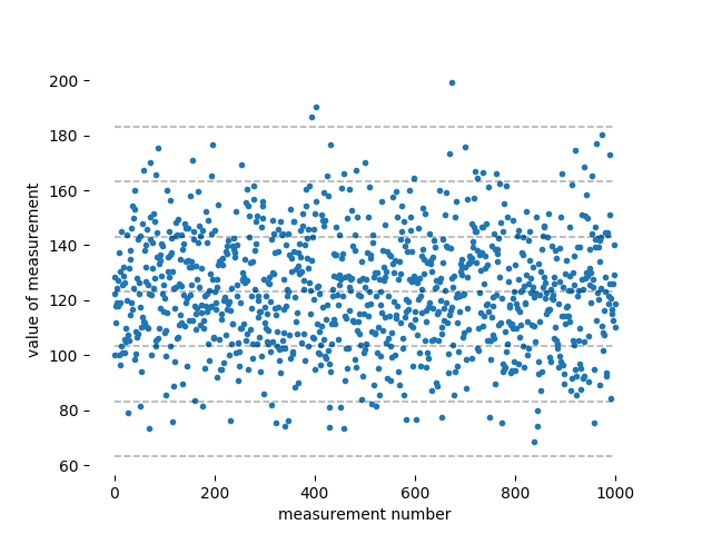
The dashed lines are at zero, $\pm1\sigma$, $\pm2\sigma$, and $\pm3\sigma$ from the mean. You can see that most of the data lie within the $\pm1\sigma$ band around the mean, and nearly all the data lie within $\pm2\sigma$. Only very rare points lie outside of the $\pm3\sigma$ band. There happen to be exactly three measurements outside of the $\pm3\sigma$ band (near the middle, and all on the side approaching 200 cm), which someone who is new to this business might take as confirmation of the statement in another answer that 99.7% of normally-distributed data points lie within $\pm3\sigma$ of the mean. But the fact that I got exactly three "outliers," and that all of the outliers happen to be on the high side, is a fluke: three three-sigma outliers per thousand points is the average over many thousands of data points, and any particular thousand data points might have a few more or less than three outliers.

If I collapse these data into a histogram, it looks like this:

histogram of data points

You can see here that a measurement of 130 cm is not uncommon at all; this data set has fifty or sixty measurements in the bin where a measurement of 130 cm would go. When you tell me $(123.2\pm20)\rm\,cm$, I hear "usually between 100 cm and 140 cm."

What's perhaps not intuitive is that you know more about the mean than you do about any particular measurement. The "standard error on the mean" goes like $\sigma/\sqrt N$, where $\sigma$ is the standard deviation of the distribution and $N$ is the number of samples that are included in the computation of the mean. For example, this dataset has $\sigma = 20\rm\,cm$ and $N=1000$, so the uncertainty on the mean is $\sigma/\sqrt N = 0.6\rm\,cm$. The actual mean I compute from these thousand data points have a mean ofis $(123.3 \pm 0.6)\rm\,cm$, which is totally consistent with the mean of 123.2 cm that I put in by hand.

To see a little more clearly the difference between the width of a distribution and the uncertainty on the mean, here are histograms of ten different sets of 1000 measurements each, generated the same way as the one above:

ten histograms

The mean of of each data set is represented with a fat blue dot. On the left, where you can see the entire distribution, you can just barely tell that not all of the means are the same. On the right, where only the means are shown, you can see that the uncertainty estimate $\sigma/\sqrt N = 0.6\rm\,cm$ looks like a good estimator of the uncertainty on the mean, since about two-thirds of the means are within one error bar of the correct value. This is like meta-statistics: doing statistics on the means and standard deviations of several data sets.

This is a general pattern with statistics: it makes more sense if you can actually play with some data where you already know some of the things you're interested in.

For example, I got average h=123.2 cm after 100 measurements, but because water is always moving the standard deviation is high, like 20 cm. In this example, can I tell that the water level h=123.2±0.1 cm or I can tell only h=120±20cm because the standard deviation is 20cm?

This is a case where actually looking at the data makes it clearer what's happening. Here's some data which has the characteristics you give: a mean of 123.2 cm, and a standard deviation of $\sigma = 20\rm\,cm$. I've assumed a normal distribution, but you can choose a different distribution if you feel like it. These thousand are plotted versus the measurement number:

1k random data points

The dashed lines are at zero, $\pm1\sigma$, $\pm2\sigma$, and $\pm3\sigma$ from the mean. You can see that most of the data lie within the $\pm1\sigma$ band around the mean, and nearly all the data lie within $\pm2\sigma$. Only very rare points lie outside of the $\pm3\sigma$ band. There happen to be exactly three measurements outside of the $\pm3\sigma$ band (near the middle, and all on the side approaching 200 cm), which someone who is new to this business might take as confirmation of the statement in another answer that 99.7% of normally-distributed data points lie within $\pm3\sigma$ of the mean. But the fact that I got exactly three "outliers," and that all of the outliers happen to be on the high side, is a fluke: three three-sigma outliers per thousand points is the average over many thousands of data points, and any particular thousand data points might have a few more or less than three outliers.

If I collapse these data into a histogram, it looks like this:

histogram of data points

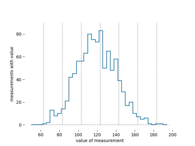
You can see here that a measurement of 130 cm is not uncommon at all; this data set has fifty or sixty measurements in the bin where a measurement of 130 cm would go. When you tell me $(123.2\pm20)\rm\,cm$, I hear "usually between 100 cm and 140 cm."

What's perhaps not intuitive is that you know more about the mean than you do about any particular measurement. The "standard error on the mean" goes like $\sigma/\sqrt N$, where $\sigma$ is the standard deviation of the distribution and $N$ is the number of samples that are included in the computation of the mean. For example, these thousand data points have a mean of $(123.3 \pm 0.6)\rm\,cm$, which is totally consistent with the mean of 123.2 that I put in by hand.

This is a general pattern with statistics: it makes more sense if you can actually play with some data where you already know some of the things you're interested in.
For example, I got average h=123.2 cm after 100 measurements, but because water is always moving the standard deviation is high, like 20 cm. In this example, can I tell that the water level h=123.2±0.1 cm or I can tell only h=120±20cm because the standard deviation is 20cm?

This is a case where actually looking at the data makes it clearer what's happening. Here's some data which has the characteristics you give: a mean of 123.2 cm, and a standard deviation of $\sigma = 20\rm\,cm$. I've assumed a normal distribution, but you can choose a different distribution if you feel like it. These thousand are plotted versus the measurement number:

1k random data points

The dashed lines are at zero, $\pm1\sigma$, $\pm2\sigma$, and $\pm3\sigma$ from the mean. You can see that most of the data lie within the $\pm1\sigma$ band around the mean, and nearly all the data lie within $\pm2\sigma$. Only very rare points lie outside of the $\pm3\sigma$ band. There happen to be exactly three measurements outside of the $\pm3\sigma$ band (near the middle, and all on the side approaching 200 cm), which someone who is new to this business might take as confirmation of the statement in another answer that 99.7% of normally-distributed data points lie within $\pm3\sigma$ of the mean. But the fact that I got exactly three "outliers," and that all of the outliers happen to be on the high side, is a fluke: three three-sigma outliers per thousand points is the average over many thousands of data points, and any particular thousand data points might have a few more or less than three outliers.

If I collapse these data into a histogram, it looks like this:

histogram of data points

You can see here that a measurement of 130 cm is not uncommon at all; this data set has fifty or sixty measurements in the bin where a measurement of 130 cm would go. When you tell me $(123.2\pm20)\rm\,cm$, I hear "usually between 100 cm and 140 cm."

What's perhaps not intuitive is that you know more about the mean than you do about any particular measurement. The "standard error on the mean" goes like $\sigma/\sqrt N$, where $\sigma$ is the standard deviation of the distribution and $N$ is the number of samples that are included in the computation of the mean. For example, this dataset has $\sigma = 20\rm\,cm$ and $N=1000$, so the uncertainty on the mean is $\sigma/\sqrt N = 0.6\rm\,cm$. The actual mean I compute from these thousand data points is $(123.3 \pm 0.6)\rm\,cm$, which is totally consistent with the mean of 123.2 cm that I put in by hand.

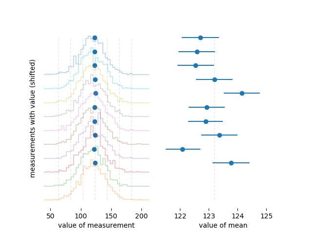
To see a little more clearly the difference between the width of a distribution and the uncertainty on the mean, here are histograms of ten different sets of 1000 measurements each, generated the same way as the one above:

ten histograms

The mean of of each data set is represented with a fat blue dot. On the left, where you can see the entire distribution, you can just barely tell that not all of the means are the same. On the right, where only the means are shown, you can see that the uncertainty estimate $\sigma/\sqrt N = 0.6\rm\,cm$ looks like a good estimator of the uncertainty on the mean, since about two-thirds of the means are within one error bar of the correct value. This is like meta-statistics: doing statistics on the means and standard deviations of several data sets.

This is a general pattern with statistics: it makes more sense if you can actually play with some data where you already know some of the things you're interested in.
Source Link
rob
  • 94.2k
  • 20
  • 177
  • 353

For example, I got average h=123.2 cm after 100 measurements, but because water is always moving the standard deviation is high, like 20 cm. In this example, can I tell that the water level h=123.2±0.1 cm or I can tell only h=120±20cm because the standard deviation is 20cm?

This is a case where actually looking at the data makes it clearer what's happening. Here's some data which has the characteristics you give: a mean of 123.2 cm, and a standard deviation of $\sigma = 20\rm\,cm$. I've assumed a normal distribution, but you can choose a different distribution if you feel like it. These thousand are plotted versus the measurement number:

1k random data points

The dashed lines are at zero, $\pm1\sigma$, $\pm2\sigma$, and $\pm3\sigma$ from the mean. You can see that most of the data lie within the $\pm1\sigma$ band around the mean, and nearly all the data lie within $\pm2\sigma$. Only very rare points lie outside of the $\pm3\sigma$ band. There happen to be exactly three measurements outside of the $\pm3\sigma$ band (near the middle, and all on the side approaching 200 cm), which someone who is new to this business might take as confirmation of the statement in another answer that 99.7% of normally-distributed data points lie within $\pm3\sigma$ of the mean. But the fact that I got exactly three "outliers," and that all of the outliers happen to be on the high side, is a fluke: three three-sigma outliers per thousand points is the average over many thousands of data points, and any particular thousand data points might have a few more or less than three outliers.

If I collapse these data into a histogram, it looks like this:

histogram of data points

You can see here that a measurement of 130 cm is not uncommon at all; this data set has fifty or sixty measurements in the bin where a measurement of 130 cm would go. When you tell me $(123.2\pm20)\rm\,cm$, I hear "usually between 100 cm and 140 cm."

What's perhaps not intuitive is that you know more about the mean than you do about any particular measurement. The "standard error on the mean" goes like $\sigma/\sqrt N$, where $\sigma$ is the standard deviation of the distribution and $N$ is the number of samples that are included in the computation of the mean. For example, these thousand data points have a mean of $(123.3 \pm 0.6)\rm\,cm$, which is totally consistent with the mean of 123.2 that I put in by hand.

This is a general pattern with statistics: it makes more sense if you can actually play with some data where you already know some of the things you're interested in.